5 Statistical physics

Statistical physics is about macroscopic systems. Classically, the state $r$ of a system of $N$ particles is represented by $2f$ real numbers

\[ \begin{align} r = \left(q_1, \dotsc, q_f;p_1, \dotsc, p_f\right) \end{align} \]

where $f$ is the number of degrees of freedom, $q_i$ is the generalized coordinates and $p_i$ is the generalized momenta. Here $\mathcal{O}\left(f\right) = \mathcal{O}\left(N\right)$. Examples of such a system would be a crystal or $10^{23}$ gas particles in a box. These examples make it clear that the microscopic state of a macroscopic system is not relevant. The exact speed of one of the $10^{23}$ particles does not matter. The microstate is therefore not of interest.

A significant simplification of the statistics is obtained if one assumes a quantum mechanical system. This is because a stationary state in quantum mechanics can be determined by a finite number of discrete quantum numbers if the system is confined in a finite volume. A microstate $r$ can then be defined by a finite number of natural numbers $n_i$,

\[ \begin{align} r = \left(n_i\right). \end{align} \]

A macrostate $M$ is defined by specifying the probabilities $P_r$ for the microstates $r$,

\[ \begin{align} M \coloneqq \left(P_r\right). \end{align} \]

To do this, imagine a number $N$ of identical systems, a so-called ensemble. This can be a mental concept to understand a single system, but it can also be $N$ actually existing systems, such as $N$ spin-containing particles. Let there be $N_r$ systems in the microstate $r$. Then you can use the $P_r$

\[ \begin{align} P_r \coloneqq\lim\limits_{N\to\infty}\frac{N_r}{N} \end{align} \]

define. Now one can assume as limiting conditions that the system is closed, i.e. that the number of particles and energy are constant. In addition, there should be no symmetries from which further restrictive conservation laws would follow. In particular, conservation of momentum and angular momentum should not apply. The density operator of the ensemble is defined by

\[ \begin{align} \newhat{\rho}\left(t\right) \coloneqq\frac{1}{N}\sum_{j = 1}^{N}\left|j\right\rangle\left\langle j\right|. \end{align} \]

Here $j$ runs over all ensemble members and $\left|j\right\rangle$ is the state of the $j-$th system. The states $\left|j\right\rangle$ do not have to be orthogonal to each other, but they must be normalized, in particular several systems can be in the same state. Let $\left(\left|\psi_k\right\rangle\right)$ for $k\geq 1$ be an orthonormal basis of the Hilbert space from which the $\left|j\right\rangle $states come. The probability $P_l$ of encountering a randomly chosen ensemble member in the state $\left|\psi_l\right\rangle$ follows

\[ \begin{align} P_l = \frac{N_l}{N} = \frac{1}{N}\sum_{j = 1}^{N}\left|\left\langle\psi_l|j\right\rangle\right|^2 = \frac{1}{N}\sum_{j = 1}^{N}\left\langle\psi_l|j\right\rangle\left\langle j|\psi_l\right\rangle = \left\langle\psi_l\left|\newhat{\rho}\right|\psi_l\right\rangle. \end{align} \]

Here, $N_r$ was interpreted as the number of systems that are encountered in a quantum mechanical measurement in the state $\left|\psi_r\right\rangle$. The macrostate $\left(P_r\right)$ can be determined from the density operator, which is why the density operator is also called statistical operator. It follows from this

\[ \begin{align} \text{tr}\left(\newhat{\rho}\right) &= 1. \end{align} \]

For an expectation value $\left\langle\newhat{A}\right\rangle$ it follows that $\newhat{A}$ is Hermitian

\[ \begin{align} \left\langle\newhat{A}\right\rangle &= \frac{1}{N}\sum_{j = 1}^{N}\left\langle j\left|\newhat{A}\right|j\right\rangle = \frac{1}{N}\sum_{j = 1}^{N}\sum_{k = 1}^{\infty}\big\langle j\big|\psi_k\big\rangle\left\langle \psi_k\left|\newhat{A}\right|j\right\rangle = \frac{1}{N}\sum_{j = 1}^{N}\sum_{k = 1}^{\infty}\left\langle \psi_k\left|\newhat{A}\right|j\right\rangle\big\langle j\big|\psi_k\big\rangle\nonumber\\ &= \sum_{k = 1}^{\infty}\Big\langle \psi_k\Big|\frac{1}{N}\sum_{j = 1}^{N}\newhat{A}\Big|j\Big\rangle\Big\langle j\Big|\psi_k\Big\rangle = \sum_{k = 1}^{\infty}\left\langle\psi_k\left|\newhat{A}\newhat{\rho}\right|\psi_k\right\rangle = \text{tr}\left(\newhat{A}\newhat{\rho}\right). \end{align} \]

Let $\left|\psi_l\right\rangle, \left|\psi_m\right\rangle$ be two states, then the following applies

\[ \begin{align} \left\langle\psi_l|\newhat{\rho}\psi_m\right\rangle &= \frac{1}{N}\langle\psi_l|\sum_{j = 1}^{N}|j\rangle\left\langle j\newvline\psi_m\right\rangle = \frac{1}{N}\sum_{j = 1}^{N}\langle\psi_l|j\rangle\left\langle j\newvline\psi_m\right\rangle = \frac{1}{N}\left(\sum_{j = 1}^{N}\langle\psi_m|j\rangle\left\langle j\newvline\psi_l\right\rangle\right)^\star\nonumber\\ &= \frac{1}{N}\left(\langle\psi_m|\sum_{j = 1}^{N}|j\rangle\left\langle j\newvline\psi_l\right\rangle\right)^\star = \left\langle\psi_m|\newhat{\rho}\psi_l\right\rangle^\star = \left\langle\newhat{\rho}\psi_l|\psi_m\right\rangle. \end{align} \]

The density operator is therefore Hermitian. The last property of the density operator to be noted here is

\[ \begin{align} \text{tr}\left(\newhat{\rho}^2\right) &= \left\langle\newhat{\rho}\right\rangle = \frac{1}{N}\sum_{j = 1}^{N}\left\langle j\left|\newhat{\rho}\right|j\right\rangle = \frac{1}{N}\sum_{j = 1}^{N}\langle j|\frac{1}{N}\sum_{j' = 1}^{N}|j'\rangle\left\langle j'|j\right\rangle\nonumber\\ &= \frac{1}{N^2}\sum_{j, j' = 1}^{N}\left|\left\langle j|j'\right\rangle\right|^2\leq 1\frac{1}{N^2}\sum_{j, j' = 1}^{N}1 = 1. \end{align} \]

So it is $\text{tr}\left(\newhat{\rho}^2\right) = 1$ if and only if all ensemble members are in the same state. This is called a pure state, otherwise it is called a mixed state.

The expected value of the Hamiltonian is the expected value of the energy or the energy $E$ for short. So it applies

\[ \begin{align} E = \text{tr}\left(\newhat{H}\newhat{\rho}\right). \end{align} \]

With the time-dependent SG follows

\[ \begin{align} i\hbar\frac{\partial\newhat{\rho}}{\partial t} &= \frac{1}{N}\sum_{i = 1}^{N}\newhat{H}\left|j\right\rangle\left\langle j\right| + \left|j\right\rangle i\hbar\frac{\partial}{\partial t}\left\langle j\right| \end{align} \]

With

\[ \begin{align} i\hbar\frac{\partial}{\partial t}\left\langle j\right| &= i\hbar\frac{\partial}{\partial t}\left| j\right\rangle^+= -\left(i\hbar\frac{\partial}{\partial t}\left| j\right\rangle\right)^+= -\left(\newhat{H}\left| j\right\rangle\right)^+= -\left\langle j\right|\newhat{H} \end{align} \]

you get

\[ \begin{align} i\hbar\frac{\partial\newhat{\rho}}{\partial t} = \left[\newhat{H}, \newhat{\rho}\right].\tag{5.14}\label{eq:von_neumann} \end{align} \]

This is the von Neumann equation.

Let a closed system be exposed to a constant perturbation operator $\newhat{v}_h$, then Eq. (4.392) for the transition rate $R_{r, r'}$ between two microstates $\left|\psi_r\right\rangle, \left|\psi_{r'}\right\rangle$

\[ \begin{align} R_{r, r'} = \frac{2\pi}{\hbar}\left|\left\langle\psi_{r}\left|\newhat{v}_h\right|\psi_{r'}\right\rangle\right|^2 = R_{r', r}. \end{align} \]

For the time derivative of the probabilities $P_r\left(t\right)$ follows

\[ \begin{align} \frac{dP_r\left(t\right)}{dt} = -\sum_{r'}^{}R_{r, r'}P_r + \sum_{r'}^{}R_{r', r}P_{r'} \end{align} \]

Eq. (15.137) is called master equation. Define

\[ \begin{align} H\left(t\right) \coloneqq\sum_{r = 1}^{\infty}P_r\ln\left(P_r\right). \end{align} \]

Then applies

\[ \begin{align} \frac{dH}{dt} &= \sum_{r}\left(\newdot{P}_r\ln\left(P_r\right) + \newdot{P}_r\right) = \frac{1}{2}\left[\sum_{r}^{}\newdot{P}_r\ln\left(eP_r\right) + \sum_{r'}\newdot{P}_{r'}\ln\left(eP_{r'}\right)\right]\nonumber\\ &= \frac{1}{2}\sum_{r, r'}^{}R_{r, r'}\left(P_{r'} - P_r\right)\left[\ln\left(eP_r\right) - \ln\left(eP_{r'}\right)\right] = \frac{1}{2}\sum_{r, r'}^{}R_{r, r'}P_r\left(1 - \frac{P_{r'}}{P_r}\right)\ln\left(\frac{P_{r'}}{P_r}\right)\tag{5.19}\label{eq:deriv_h_theorem} \end{align} \]

$R_{r, r'}P_r\geq 0$ as well apply

\[ \begin{align} \left(1 - x\right)\ln\left(x\right)\leq 0. \end{align} \]

Therefore applies

\[ \begin{align} \frac{dH}{dt}\leq 0.\tag{5.21}\label{eq:h_theorem} \end{align} \]

Eq. (5.21) is called H-theorem. The equilibrium state is defined as the state with constant $P_r$, i.e. with $\newdot{H} = 0$ or $H = $ minimal. We further define the entropy $S$ by

\[ \begin{align} S \coloneqq - k_BH \end{align} \]

What can be said about entropy is:

5.1 Microcanonical ensemble

According to Eq. (5.19) holds in equilibrium

\[ \begin{align} P_{r} = P_{r'} \end{align} \]

for all $r, r'$ with $E_r = E_{r'}$. In a closed system, by definition, only states with $E_r = E$ can be achieved.

You can now measure the energy $E$ of the system, with an accuracy $\delta E\gg \Delta E_r$, where $\Delta E_r$ represents a typical distance between the energy levels of the system. The fact that an energy $E$ was measured with the precision $\delta E$ should be interpreted as meaning that the true energy $E'$ of the system lies in the interval $\left[E - \delta E, E\right)$. There are therefore a number of states $r$ whose energies $E_r$ lie in this interval and are therefore compatible with the measurement. One defines the microcanonical partition function $\Omega$ by

\[ \begin{align} \Omega\left(E, x\right) \coloneqq \sum_{r:E - \delta E\leq E_r< E}^{}1. \end{align} \]

Here $x$ denotes all parameters other than the energy that define the system macroscopically, in particular the volume. Since all accessible microstates are equally probable,

\[ \begin{align} P_r = \frac{1}{\Omega\left(E, x\right)}\cdot\begin{cases} 1, \:E - \delta E\leq E_r < E,\\ 0, \text{ sonst} \end{cases}\tag{5.25}\label{eq:mikrokan_ens} \end{align} \]

In the microcanonical ensemble, to which the microcanonical partition function refers, all systems are closed and have the same energies and particle numbers. So these are very specific physical requirements. In this case the entropy follows

\[ \begin{align} S\left(E, x\right) = -k_B\sum_{r = 1}^{\infty}\frac{1}{\Omega\left(E, x\right)}\ln\left(\frac{1}{\Omega\left(E, x\right)}\right) = k_B\ln\left[\Omega\left(E, x\right)\right].\tag{5.26}\label{eq:entropie_mikrokanonisch} \end{align} \]

The energy of a system can be written with reference to an orthonormal basis $\left(\left|\psi_k\right\rangle\right)$ from eigenstates of the Hamiltonian

\[ \begin{align} E = \sum_{k = 1}^{\infty}P_kE_k\left(x\right). \end{align} \]

For the change in energy follows in linear order

Here, a partial derivative was simply noted for the derivative with respect to $x$, in general it is a sum of several partial derivatives, and $E_k = E$ was also used. Heat means a change in the occupation probabilities with constant external parameters $x$, Work means a change in the energy due to a change in the external parameters; these are conceptual definitions. A differential $df$ is a shorthand notation for a linear Taylor expansion of $f$ ignoring the error term. Since the energy $E$ as a state variable does not depend on the process that led to the state, o. B. d. A. a quasi-static processThe word quasi can be translated as almost. can be assumed:

\[ \begin{align} dE = dQ_{\text{qs}} - dW_{\text{qs}}\tag{5.29}\label{eq:td_1_0} \end{align} \]

In such a process a sequence of equilibrium states is passed through; one can imagine it as an infinitely slow process. Furthermore, for each external parameter $x_i$ one defines a generalized force $X_i$ by

\[ \begin{align} X_i \coloneqq - \sum_{k = 1}^{\infty}P_k\frac{\partial E_k\left(x\right)}{\partial x_i}.\tag{5.30}\label{eq:def_gen_kraft} \end{align} \]

In equilibrium this becomes

\[ \begin{align} X_i = -\frac{\partial E\left(x\right)}{\partial x_i}. \end{align} \]

In the case of a quasi-static process, the following applies:

\[ \begin{align} dW_{\text{qs}} = -\sum_{i}^{}\frac{\partial E\left(x\right)}{\partial x_i}dx_i = \sum_{i}^{}X_idx_i.\tag{5.32}\label{eq:work_qs} \end{align} \]

The pressure $p$ is the generalized force of the volume:

\[ \begin{align} p\left(E, x\right) \coloneqq - \sum_{k = 1}^{\infty}P_k\frac{\partial E_k\left(x\right)}{\partial V} \end{align} \]

In the case $x = V$, when the only external parameter is the volume, it follows

The temperature $T$ is given by

\[ \begin{align} \frac{1}{T} \coloneqq \frac{\partial S\left(E, x\right)}{\partial E}\tag{5.35}\label{eq:def_temperatur} \end{align} \]

defined, you continue to lay

\[ \begin{align} \beta \coloneqq\frac{1}{k_BT} \end{align} \]

as an abbreviation. Eq. (5.30) is unwieldy because it has to be averaged over an infinite number of quantum mechanical states. To derive an alternative formula, one starts from the microcanonical partition function

\[ \begin{align} \Omega\left(E, x\right) = \Omega\left(E, x_1, x_i\right) = \sum_{r:E - \delta E\leq E_r

from, here $x_i$ stands for all external parameters except $x_1$, where $x_1$ is chosen arbitrarily. It applies

\[ \begin{align} \frac{\partial\ln\left[\Omega\left(E, x\right)\right]}{\partial x_1} &= \frac{\ln\left[\Omega\left(E, x_1 + dx_1, x_i\right)\right] - \ln\left[\Omega\left(E, x_1, x_i\right)\right]}{dx_1}. \end{align} \]

Now you do the math

\[ \begin{align} \Omega\left(E, x_1 + dx_1, x_i\right) &= \sum_{r:E - \delta E\leq E_r\left(x_1 + dx_1, x_i\right)

with

\[ \begin{align} dE_r = \frac{\partial E_r}{\partial x_1}dx_1. \end{align} \]

One can

\[ \begin{align} dE_r = \newoverline{dE_r} \end{align} \]

set, whereby the averaging takes place over all microstates of the equilibrium state:

\[ \begin{align} \Omega\left(E, x_1 + dx_1, x_i\right) &= = \sum_{r:E - \newoverline{dE_r} - \delta E\leq E_r\left(x\right)

Because of

\[ \begin{align} X_i = -\newoverline{\frac{\partial E}{\partial x_i}} \end{align} \]

is

\[ \begin{align} \newoverline{dE_r} = -X_1x_1. \end{align} \]

Therefore applies

\[ \begin{align} \frac{\partial\ln\left[\Omega\left(E, x\right)\right]}{\partial x_1} &= -\frac{\ln\left[\Omega\left(E - \newoverline{dE_r}, x\right)\right] - \ln\left[\Omega\left(E, x\right)\right]}{\newoverline{dE_r}/X_1} = \frac{\partial\ln\left[\Omega\left(E, x\right)\right]}{\partial E}X_1 = \beta X_1\nonumber\\ \Rightarrow X_i &= T\frac{\partial S\left(E, x\right)}{\partial x_i}. \end{align} \]

For printing follows

\[ \begin{align} p = T\frac{\partial S\left(E, x\right)}{\partial V}\tag{5.46}\label{eq:pressure_prop_0} \end{align} \]

For the change in entropy applies

If two systems $A, B$ with the microcanonical partition sums $\Omega_A\left(E_A, x_A\right)$ and $\Omega_E\left(E_B, x_B\right)$ are in equilibrium, then the energy $E$ of the entire system applies

\[ \begin{align} E = E_A + E_B. \end{align} \]

For the partition function $\Omega\left(E, x\right)$ of the entire system follows

\[ \begin{align} \Omega\left(E, x\right) = \Omega_A\left(E_A, x_A\right)\Omega_B\left(E_B, x_B\right). \end{align} \]

The partition sums of the subsystems must be multiplied because all combinations of microstates can occur. For the entropy $S$ of the entire system follows

\[ \begin{align} S\left(E, x\right) = k_B\ln\left[\Omega_A\left(E_A, x_A\right)\right] + k_B\ln\left[\Omega_B\left(E_B, x_B\right)\right] = S_A\left(E_A, x_A\right) + S_B\left(E - E_A, x_B\right). \end{align} \]

So the entropy is additive. At equilibrium it is maximum:

\[ \begin{align} \frac{\partial S}{\partial E_A} = 0\Rightarrow\frac{\partial S_A}{\partial E_A} + \frac{\partial S_B}{\partial E_A} = \frac{\partial S_A}{\partial E_A} - \frac{\partial S_B}{\partial E_B} = 0\Rightarrow T_A = T_B\tag{5.52}\label{eq:t_gleichgewicht} \end{align} \]

If the systems $A, B$ are also in $x_i-$exchange, one obtains the condition under the assumption $x_{i} = x_{i, A} + x_{i, B}$

\[ \begin{align} \nabla S = 0\Rightarrow \frac{\partial S}{\partial x_{i, A}} = 0\Rightarrow \frac{\partial S_A}{\partial x_{i, A}} + \frac{\partial S_B}{\partial x_{i, A}} = \frac{\partial S_A}{\partial x_{i, A}} - \frac{\partial S_B}{\partial x_{i, B}} = 0. \end{align} \]

From this, under the assumption $T_A = T_B$, the equality of the generalized forces follows

An equation of the form

\[ \begin{align} p = p\left(T, V, N\right) \end{align} \]

is called thermal equation of state, while equations of the form

\[ \begin{align} E = E\left(T, V, N\right) \end{align} \]

can be referred to as caloric equation of state. At this point we refer to the notation usual in thermodynamics

\[ \begin{align} \frac{\partial f\left(x, y, z\right)}{\partial x} = \left(\frac{\partial f}{\partial x}\right)_{y, z} \end{align} \]

for partial derivatives. The heat capacity of a substance is defined by

\[ \begin{align} C^{(p)} \coloneqq \left(\frac{dQ_{\text{qs}}}{dT}\right)_{p} \end{align} \]

or

\[ \begin{align} C^{(V)} \coloneqq \left(\frac{dQ_{\text{qs}}}{dT}\right)_{V}, \end{align} \]

depending on whether the pressure or the volume is kept constant during the process. With Eq. (5.48) follows

\[ \begin{align} C^{(p)} &= T\left(\frac{\partial S}{\partial T}\right)_p, \tag{5.60}\label{eq:waermekap_p_entropie}\\ C^{(V)} &= T\left(\frac{\partial S}{\partial T}\right)_V\tag{5.61}\label{eq:waermekap_v_entropie}. \end{align} \]

The specific heat capacity of a system with mass $m$ is defined by

\[ \begin{align} c^{(p)} \coloneqq \frac{1}{m}C^{(p)} \end{align} \]

and analogously for $c^{(V)}$.

5.2 Canonical and grand canonical ensemble

The canonical ensemble consists of systems $A$ that are in heat exchange with large surrounding systems $B$, so-called bath systems. However, there is no particle or xi exchange. The entire system consisting of $A$ and $B$ is complete so that the microcanonical ensemble can be used. Then applies to the total energy

\[ \begin{align} E = E_A + E_B = \text{const}. \end{align} \]

For the microcanonical partition sums $\Omega$ of the entire system applies

\[ \begin{align} \Omega = \Omega\left(E, x\right). \end{align} \]

The entire system is equally likely to be found in each of its accessible microstates. The number of states $n\left(E_A\right)$ with a fixed energy $E_A$ of the system $A$ is given by

\[ \begin{align} n\left(E_A\right) = \Omega_A\left(E_A, x_A\right)\Omega_B\left(E_B, x_B\right), \end{align} \]

where $\Omega_A$ is the microcanonical partition function of system $A$ and $\Omega_B$ is that of system $B$. The probability of encountering a state $r$ with an energy $E_r = E_A$ in the system $A$ is the probability

\[ \begin{align} P\left(E_A\right) = \frac{n_A}{\Omega\left(E, x\right)} = \frac{\Omega_A\left(E_A, x_A\right)\Omega_B\left(E_B, x_B\right)}{\Omega\left(E, x\right)}, \end{align} \]

to find the system $A$ at an energy $E_A$, divided by the number of these equally probable states:

\[ \begin{align} P_r = \frac{P\left(E_A\right)}{\Omega_A\left(E_A, x_A\right)} = \frac{\Omega_B\left(E - E_A, x - x_A\right)}{\Omega\left(E, x\right)} \end{align} \]

$E_B = E - E_A$ and $x_B = x - x_A$ were used. Because of $E_B\gg E_A$ you can expand the counter according to $E_A$ around $E_A = 0$:

\[ \begin{align} \ln\left[\Omega_B\left(E - E_A, x - x_A\right)\right] = \ln\left[\Omega_B\left(E, x - x_A\right)\right] - \beta E_A + \mathcal{O}\left(E_A^2\right) \end{align} \]

There is

\[ \begin{align} \beta = \frac{1}{k_BT_K} \end{align} \]

with the temperature of the heat bath, which is equal to the temperature $T$ of the entire system, since this is in equilibrium (see equation (5.223)). Neglecting the higher order terms:

\[ \begin{align} P_r = \frac{\Omega_B\left(E, x - x_A\right)}{\Omega\left(E, x\right)}e^{-\beta E_r} = \frac{1}{Z}e^{-\beta E_r}. \end{align} \]

$Z = \frac{\Omega\left(E, x - x_A\right)}{\Omega_B\left(E, x\right)}$ is the canonical partition function, which acts as a normalization constant and represents

\[ \begin{align} \sum_{r}^{}P_r = 1 \end{align} \]

secure:

In the grand canonical ensemble, not only heat but also particle exchange is possible with the system $B$. Then additionally applies

\[ \begin{align} N = N_A + N_B = \text{const}. \end{align} \]

for the particle number. For the number of states $n\left(E_A, N_A\right)$ in which the system $A$ has the energy $E_A$ and the particle number $N_A$, applies

\[ \begin{align} n\left(E_A, N_A\right) = \Omega_A\left(E_A, N_A, x_A\right)\Omega_B\left(E_B, N_B, x_B\right). \end{align} \]

The probability $P\left(E_A, N_A\right)$ of finding a state $r$ with the energy $E_r = E_A$ and the particle number $N_r = N_A$ in the system $A$ is given by the probability

\[ \begin{align} P\left(E_A, N_A\right) &= \frac{n\left(E_A, N_A\right)}{\Omega\left(E, x\right)} = \frac{\Omega_A\left(E_A, N_A, x_A\right)\Omega_B\left(E_B, N_B, x_B\right)}{\Omega\left(E, x\right)}, \end{align} \]

to find the system $A$ with an energy $E_A$ and particle number $N_A$, divided by the number of these equally probable states:

\[ \begin{align} P_r = \frac{P\left(E_A, N_A\right)}{\Omega_A\left(E_A, N_A, x_A\right)} = \frac{\Omega_B\left(E - E_A, N - N_A, x_B\right)}{\Omega\left(E, x\right)} \end{align} \]

$E_B = E - E_A$, $N_B = N - N_A$ and $x_B = x - x_A$ were used. Because of $E_B\gg E_A$ and $N_B\gg N_A$ you can develop the counter again:

\[ \begin{align} \ln\left[\Omega_B\left(E - E_A, N - N_A, x - x_A\right)\right] &= \ln\left[\Omega_B\left(E, N, x - x_A\right)\right] - \beta E_A - \frac{1}{k_B}\frac{\partial S}{\partial N}N_A\nonumber\\ & + \mathcal{O}\left(E_A^2, N_A^2, E_AN_A\right). \end{align} \]

The negative generalized force of the particle number is defined by the chemical potential

Neglecting the higher order terms, we therefore have:

\[ \begin{align} P_r = \frac{\Omega_B\left(E, N, x - x_A\right)}{\Omega\left(E, x\right)}e^{-\beta\left(E_r - \mu N_r\right)} = \frac{1}{Y}e^{-\beta\left(E_r - \mu N_r\right)} \end{align} \]

$Y = \frac{\Omega\left(E, x\right)}{\Omega_B\left(E, N, x - x_A\right)}$ is the grand canonical partition function, which acts as a normalization constant and represents

\[ \begin{align} \sum_{r}^{}P_r = 1 \end{align} \]

secure:

Now the first law should be generalized to the case $dN \not= 0$. With the equations (5.29) and (5.32) follows

\[ \begin{align} dE = dQ_{\text{qs}} - dW_{\text{qs}} = dQ_{\text{qs}} - \sum_{i}X_idx_i = dQ_{\text{qs}} - \frac{\partial E}{\partial V}dV - \frac{\partial E}{\partial N}dN = dQ_{\text{qs}} - pdV + \mu dN.\tag{5.82}\label{eq:td_1_id_gas} \end{align} \]

5.2.1 Thermodynamic potentials

A thermodynamic potential is a state variable from which all state variables can be determined by partial differentiation. In this section, only the volume $V$ and the particle number $N$ are considered as external parameters. In addition to the energy, the following thermodynamic potentials are defined:

For the differentials it follows that $dE = dQ - pdV + \mu dN$

\[ \begin{align} dF &= -SdT - pdV + \mu dN, \tag{5.87}\label{eq:diff_free_energie}\\ dH &= TdS + Vdp + \mu dN,\\ dG &= -SdT + Vdp + \mu dN,\\ dJ &= -SdT - pdV - Nd\mu. \end{align} \]

The following statements can be seen from this:

\[ \begin{align} \left(\frac{\partial E}{\partial S}\right)_{V, N} = T, & {} & \left(\frac{\partial E}{\partial V}\right)_{S, N} = -p, & {} & \left(\frac{\partial E}{\partial N}\right)_{S, V} &= \mu\tag{5.91}\label{eq:chemisches_potential_prop_0}\\ \end{align} \] \[ \begin{align} \left(\frac{\partial F}{\partial T}\right)_{V, N} = -S, & {} & \left(\frac{\partial F}{\partial V}\right)_{T, N} = -p, & {} & \left(\frac{\partial F}{\partial N}\right)_{T, V} = \mu \end{align} \] \[ \begin{align} \left(\frac{\partial H}{\partial S}\right)_{p, N} = T, & {} & \left(\frac{\partial H}{\partial p}\right)_{S, N} = V, & {} & \left(\frac{\partial H}{\partial N}\right)_{S, p} = \mu \end{align} \] \[ \begin{align} \left(\frac{\partial G}{\partial T}\right)_{p, N} = -S, & {} & \left(\frac{\partial G}{\partial p}\right)_{T, N} = V, & {} & \left(\frac{\partial G}{\partial N}\right)_{T, p} = \mu\tag{5.95}\label{eq:chemisches_potential_prop_2} \end{align} \] \[ \begin{align} \left(\frac{\partial J}{\partial T}\right)_{V, \mu} = -S, & {} & \left(\frac{\partial J}{\partial V}\right)_{T, \mu} = -p, & {} & \left(\frac{\partial J}{\partial\mu}\right)_{T, V} = -N \end{align} \]

These are three statements each for the partial derivatives of $E$, $F$, $H$, $G$ and $J$. By applying the equality of the second partial derivatives, 15 non-trivial thermodynamic relations can be derived, which are called Maxwell relations:

\[ \begin{align} \left(\frac{\partial^2E}{\partial V\partial S}\right)_N = \left(\frac{\partial^2E}{\partial S\partial V}\right)_N&\Rightarrow\left(\frac{\partial T}{\partial V}\right)_{S, N} = -\left(\frac{\partial p}{\partial S}\right)_{V, N}\\ \left(\frac{\partial^2E}{\partial N\partial S}\right)_V = \left(\frac{\partial^2E}{\partial S\partial N}\right)_V&\Rightarrow\left(\frac{\partial T}{\partial N}\right)_{S, V} = \left(\frac{\partial \mu}{\partial S}\right)_{N, V} \end{align} \] \[ \begin{align} \left(\frac{\partial^2E}{\partial N\partial V}\right)_S = \left(\frac{\partial^2E}{\partial V\partial N}\right)_S&\Rightarrow -\left(\frac{\partial p}{\partial N}\right)_{V, S} = \left(\frac{\partial \mu}{\partial V}\right)_{N, S}\\ \left(\frac{\partial^2F}{\partial V\partial T}\right)_N = \left(\frac{\partial^2F}{\partial T\partial V}\right)_N&\Rightarrow\left(\frac{\partial S}{\partial V}\right)_{T, N} = \left(\frac{\partial p}{\partial T}\right)_{V, N} \end{align} \] \[ \begin{align} \left(\frac{\partial^2F}{\partial N\partial T}\right)_V = \left(\frac{\partial^2F}{\partial T\partial N}\right)_V&\Rightarrow -\left(\frac{\partial S}{\partial N}\right)_{T, V} = \left(\frac{\partial\mu}{\partial T}\right)_{N, V}\tag{5.101}\label{eq:maxwell_rel_4}\\ \left(\frac{\partial^2F}{\partial N\partial V}\right)_T = \left(\frac{\partial^2F}{\partial V\partial N}\right)_T&\Rightarrow -\left(\frac{\partial p}{\partial N}\right)_{V, T} = \left(\frac{\partial\mu}{\partial V}\right)_{N, T} \end{align} \] \[ \begin{align} \left(\frac{\partial^2H}{\partial p\partial S}\right)_N = \left(\frac{\partial^2H}{\partial S\partial p}\right)_N&\Rightarrow\left(\frac{\partial T}{\partial p}\right)_{S, N} = \left(\frac{\partial V}{\partial S}\right)_{p, N}\\ \left(\frac{\partial^2H}{\partial N\partial S}\right)_p = \left(\frac{\partial^2H}{\partial S\partial N}\right)_p&\Rightarrow\left(\frac{\partial T}{\partial N}\right)_{S, p} = \left(\frac{\partial\mu}{\partial S}\right)_{N, p} \end{align} \] \[ \begin{align} \left(\frac{\partial^2H}{\partial N\partial p}\right)_S = \left(\frac{\partial^2H}{\partial p\partial N}\right)_S&\Rightarrow\frac{V}{N} = \left(\frac{\partial V}{\partial N}\right)_{p, S} = \left(\frac{\partial\mu}{\partial p}\right)_{N, S}\tag{5.105}\label{eq:maxwell_rel_1}\\ \left(\frac{\partial^2G}{\partial p\partial T}\right)_N = \left(\frac{\partial^2G}{\partial T\partial p}\right)_N&\Rightarrow -\left(\frac{\partial S}{\partial p}\right)_{T, N} = \left(\frac{\partial V}{\partial T}\right)_{p, N} \end{align} \] \[ \begin{align} \left(\frac{\partial^2G}{\partial N\partial T}\right)_p = \left(\frac{\partial^2G}{\partial T\partial N}\right)_p&\Rightarrow -\frac{S}{N} = -\left(\frac{\partial S}{\partial N}\right)_{T, p} = \left(\frac{\partial\mu}{\partial T}\right)_{N, p}\tag{5.107}\label{eq:maxwell_rel_2}\\ \left(\frac{\partial^2G}{\partial N\partial p}\right)_T = \left(\frac{\partial^2G}{\partial p\partial N}\right)_T&\Rightarrow\left(\frac{\partial V}{\partial N}\right)_{p, T} = \left(\frac{\partial\mu}{\partial p}\right)_{N, T}\tag{5.108}\label{eq:maxwell_rel_3} \end{align} \] \[ \begin{align} \left(\frac{\partial^2J}{\partial T\partial V}\right)_\mu = \left(\frac{\partial^2J}{\partial V\partial T}\right)_\mu&\Rightarrow\left(\frac{\partial p}{\partial T}\right)_{\mu, V} = \left(\frac{\partial S}{\partial V}\right)_{\mu, T}\\ \left(\frac{\partial^2J}{\partial T\partial \mu}\right)_V = \left(\frac{\partial^2J}{\partial \mu\partial T}\right)_V&\Rightarrow\left(\frac{\partial N}{\partial T}\right)_{\mu, V} = \left(\frac{\partial S}{\partial\mu}\right)_{T, V} \end{align} \] \[ \begin{align} \left(\frac{\partial^2J}{\partial V\partial\mu}\right)_T = \left(\frac{\partial^2J}{\partial\mu\partial V}\right)_T&\Rightarrow\left(\frac{\partial N}{\partial V}\right)_{\mu, T} = \left(\frac{\partial p}{\partial\mu}\right)_{T, V}\tag{5.111}\label{eq:maxwell_rel_0} \end{align} \]

If you know the microscopic structure of a system, you can determine the entropy, the microcanonical partition function or the grand canonical partition function, depending on the physical requirements. The question is how one can determine macroscopic quantities such as compressibilities or heat capacities from the partition sums. To do this, one must be able to express one of the thermodynamic potentials in terms of the partition function of the system. First, the canonical ensemble is considered. In this case $\left(T, V, N\right)$ or alternatively $\left(\beta, V, N\right)$ are fixed. It applies

\[ \begin{align} d\ln\left[Z\left(\beta, V, N\right)\right] = \frac{\partial\ln\left(Z\right)}{\partial\beta}d\beta + \frac{\partial\ln\left(Z\right)}{\partial V}dV + \frac{\partial\ln\left(Z\right)}{\partial N}dN. \end{align} \]

Now the partial derivatives of the partition function Eq. (5.72) calculated:

\[ \begin{align} \frac{\partial\ln\left(Z\right)}{\partial\beta} &= -\frac{1}{Z}\sum_{r}^{}E_r\exp\left(-\beta E_r\right) = -E\\ \frac{\partial\ln\left(Z\right)}{\partial V} &= -\frac{\beta}{Z}\sum_r\frac{\partial E_r\left(V, N\right)}{\partial V}\exp\left(-\beta E_r\right) = -\beta\newoverline{\frac{\partial E_r}{\partial V}} = \beta p \end{align} \] \[ \begin{align} \frac{\partial\ln\left(Z\right)}{\partial N} &= -\frac{\beta}{Z}\sum_r\frac{\partial E_r\left(V, N\right)}{\partial N}\exp\left(-\beta E_r\right) = -\beta\newoverline{\frac{\partial E_r}{\partial N}} = -\beta\mu \end{align} \]

It therefore applies

\[ \begin{align} d\ln\left(Z\left(\beta, V, N\right)\right) &= -Ed\beta + \beta pdV - \beta\mu dN\nonumber\\ \Rightarrow d\left(\ln\left(Z\right) + \beta E\right) &= \beta\left(dE + pdV - \mu dN\right) = \frac{1}{k_B}\left(\frac{dE}{T} + \frac{p}{T}dV - \frac{\mu}{T}dN\right) \end{align} \]

By comparing with Eq. (5.47) is obtained

\[ \begin{align} k_Bd\left[\ln\left(Z\right) + \beta E\right] &= dS\Rightarrow S = k_B\left[\ln\left(Z\right) + \beta E\right] + C. \end{align} \]

The constant $C$ results in zero, which will not be shown here, so it follows

In the grand canonical ensemble $\left(T, V, \mu\right)$ are fixed, the differential is obtained

\[ \begin{align} d\ln\left[Y\left(\beta, V, \mu\right)\right] = \frac{\partial\ln\left(Y\right)}{\partial\beta}d\beta + \frac{\partial\ln\left(Y\right)}{\partial V}dV + \frac{\partial\ln\left(Y\right)}{\partial\mu}d\mu. \end{align} \]

The partial derivatives are calculated using the partition function Eq. (5.81)

\[ \begin{align} \frac{\partial\ln\left(Y\right)}{\partial\beta} &= -\frac{1}{Y}\sum_{r}^{}\left(E_r - \mu N_r\right)\exp\left(-\beta \left(E_r - \mu N_r\right)\right) = -E + \mu N,\\ \frac{\partial\ln\left(Y\right)}{\partial V} &= -\frac{\beta}{Y}\sum_r\frac{\partial E_r\left(V, N\right)}{\partial V}\exp\left(-\beta \left(E_r - \mu N_r\right)\right) = -\beta\newoverline{\frac{\partial E_r}{\partial V}} = \beta p, \end{align} \] \[ \begin{align} \frac{\partial\ln\left(Y\right)}{\partial \mu} &= \frac{\beta}{Y}\sum_r N_r\exp\left(-\beta \left(E_r - \mu N_r\right)\right) = \beta\newoverline{N_r} = \beta N. \end{align} \]

It is thus

\[ \begin{align} d\ln\left[Y\left(\beta, V, \mu\right)\right] &= \left(-E + \mu N\right)d\beta + \beta pdV + \beta Nd\mu\nonumber\\ \Leftrightarrow d\left[\ln\left(Y\right) + \beta E - \beta\mu N\right] &= \beta\left(dE + pdV - \mu dN\right) = \frac{dS}{k_B}. \end{align} \]

This applies

\[ \begin{align} S = k_B\left[\ln\left(Y\right) + \beta E - \beta\mu N\right]\Leftrightarrow k_BT\ln\left(Y\right) = TS - E + \mu N. \end{align} \]

A possible constant here is also zero. By comparing with Eq. (5.86) follows

The equations (5.118) and (5.125) provide a connection between microscopic statistics and macroscopic thermodynamics.

For the complete differential $d\mu$ of the chemical potential $\mu = \mu\left(T, p\right)$ holds

\[ \begin{align} d\mu = \left(\frac{\partial\mu}{\partial T}\right)_pdT + \left(\frac{\partial\mu}{\partial p}\right)_Tdp \stackrel{\href{#eq:maxwell_rel_4}{\text{Glg.en (5.101), (5.108)}}}{=} -\left(\frac{\partial S}{\partial N}\right)_{T, V}dT + \left(\frac{\partial V}{\partial N}\right)_{p, T}dp. \end{align} \]

With

\[ \begin{align} \left(\frac{\partial S}{\partial N}\right)_{T, V} = \frac{S}{N} =: s, & {} & \left(\frac{\partial V}{\partial N}\right)_{p, T} = \frac{V}{N} =: v \end{align} \]

follows

which is called Gibbs-Duhem relation.

5.3 Ideal gas

An ideal gas is a gas in which the particles do not interact with each other. The Hamiltonian of an ideal gas made of $N$ particles is

\[ \begin{align} \newhat{H} = \sum_{i = 1}^{N} - \frac{\hbar^2}{2m}\Delta_i + V\left(\mathbf{r}_i\right) = \sum_{i = 1}^{N}\newhat{H}_i, \end{align} \]

it is a superposition of one-particle Hamiltonians

\[ \begin{align} \newhat{H}_i = -\frac{\hbar^2}{2m}\Delta_i + V\left(\mathbf{r}_i\right). \end{align} \]

$V\left(\mathbf{r}_i\right)$ ist das bekannte Wandpotential

\[ \begin{align} V\left(\mathbf{r}_i\right) = \begin{cases} 0, \:\mathbf{r}_i\in V,\\ \infty, \text{ sonst}, \end{cases} \end{align} \]

where $V$ is the volume to which the particles are confined. Here $V = L^3$ is a cube with edge length $L$. This corresponds to a 3D potential well, see section 4.2. The one-particle solution is

\[ \begin{align} \psi\left(\mathbf{r}_i\right)\propto\sin\left(k_{3i - 2}x\right)\sin\left(k_{3i - 1}y\right)\sin\left(k_{3i}z\right). \end{align} \]

The boundary condition applies here for $k_{3i - 2}, k_{3i - 1}, k_{3i}$

\[ \begin{align} \frac{Lp_i}{\hbar} = k_iL = n_i\pi\tag{5.133}\label{eq:deriv_ideal_gas_bc} \end{align} \]

with $n_i\in \mathbb {N}$ with $n\geq 1$. $p_i = \hbar k_i$ is the momentum. The particles do not penetrate the wall, so they have no potential energy. This therefore applies to the total energy of the system

\[ \begin{align} E = \frac{1}{2m}\sum_{i = 1}^{3N}p_i^2. \end{align} \]

To determine the microcanonical state sum of the ideal gas, one assumes $\delta E = E$:

\[ \begin{align} \Omega\left(E, V, N\right) &= \sum_{E_r

Because $\newoverline{n_i}\gg 1$, the sums were replaced by integrals in the last step. The factor $1/2^{3N}$ arises from the inclusion of negative values ​​in the integration (there are $3N$ coordinate axes that must be halved). Eq. (5.133) is implied

\[ \begin{align} dn_i = \frac{L}{\hbar\pi}dp_i. \end{align} \]

It follows

\[ \begin{align} \Omega\left(E, V, N\right) &= \left(\frac{L}{2\hbar\pi}\right)^{3N}\underbrace{\int\dotsc\int}_{\sum p_i^2< 2mE}dp_1\dotsc dp_{3N} = \frac{V^N}{\left(2\hbar\pi\right)^{3N}}\underbrace{\int\dotsc\int}_{\sum p_i^2< 2mE}dp_1\dotsc dp_{3N}. \end{align} \]

The remaining 3N-dimensional integral is the volume of a 3N-dimensional sphere of radius $\sqrt{2mE}$, so Eq. (B.143) can be used:

\[ \begin{align} \Omega\left(E, V, N\right) &= \frac{V^N}{\left(2\hbar\pi\right)^{3N}}\frac{\pi^{3N/2}}{\Gamma\left(\frac{3N}{2} + 1\right)}\sqrt{2mE}^{3N} \stackrel{\href{ch-39-derivations-of-some-mathematical-formula.html#eq:gamma_prop_1}{\text{Glg. (A.111)}}}{=} \frac{V^N}{\left(2\pi\hbar\right)^{3N}}\frac{\pi^{3N/2}}{\left(3N/2\right)!}\left(2m\right)^{3N/2}E^{3N/2}\nonumber\\ &= \frac{V^N}{\left(2\pi\hbar\right)^{3N}}\frac{1}{\left(3N/2\right)!}\left(2m\pi\right)^{3N/2}E^{3N/2} = \left[\frac{2\pi m}{\left(2\pi\hbar\right)^2}\right]^{3N/2}\frac{E^{3N/2}}{\left(3N/2\right)!}V^N \end{align} \]

Using the Stirling formula Eq. (A.117) is obtained

\[ \begin{align} \Omega\left(E, V, N\right) &= \left[\frac{2\pi m}{\left(2\pi\hbar\right)^2}\right]^{3N/2}E^{3N/2}V^N\frac{1}{\left(3N/2\right)!} \approx \sqrt{\frac{1}{2\pi}}\left[\frac{2\pi m}{\left(2\pi\hbar\right)^2}\right]^{3N/2}e^{3N/2}\left(\frac{2}{3N}\right)^{\frac{3N}{2} + \frac{1}{2}}E^{3N/2}V^N\nonumber\\ &= \frac{1}{\sqrt{3N\pi}}\left[\frac{2\pi me}{\left(2\pi\hbar\right)^2}\right]^{3N/2}\left(\frac{2}{3N}\right)^{\frac{3N}{2}}E^{3N/2}V^N = \frac{1}{\sqrt{3\pi N}}\left[\frac{4\pi me}{3\left(2\pi\hbar\right)^2}\right]^{3N/2}V^N\left(\frac{E}{N}\right)^{3N/2}. \end{align} \]

This result is not yet correct; an important modification still needs to be made. The $N$ particles are quantum mechanically indistinguishable, which means that swapping two particles changes nothing. So $N!$ states are the same, which is why one

\[ \begin{align} \Omega\to\frac{\Omega}{N!} \end{align} \]

needs to be replaced. From this it follows, again using the Stirling formula,

\[ \begin{align} \Omega\left(E, V, N\right) &= \frac{1}{\sqrt{6\pi^2}}\frac{1}{N}\left[\frac{4\pi me^{5/3}}{3\left(2\pi\hbar\right)^2}\right]^{3N/2}\left(\frac{V}{N}\right)^N\left(\frac{E}{N}\right)^{3N/2}\nonumber\\ &= \frac{1}{\sqrt{6\pi^2}}\frac{1}{N}\left[\frac{me^{5/3}}{3\pi\hbar^2}\right]^{3N/2}\left(\frac{V}{N}\right)^N\left(\frac{E}{N}\right)^{3N/2}. \end{align} \]

For the entropy follows

\[ \begin{align} \frac{S\left(E, V, N\right)}{k_B} &= \frac{1}{2}\ln\left(\frac{1}{6\pi^2}\right) - \ln\left(N\right) + \frac{3N}{2}\ln\left(c\right) + N\ln\left(\frac{V}{N}\right) + \frac{3N}{2}\ln\left(\frac{E}{N}\right)\nonumber\\ &\approx \frac{3N}{2}\ln\left(c\right) + N\ln\left(\frac{V}{N}\right) + \frac{3N}{2}\ln\left(\frac{E}{N}\right) - \ln\left(N\right)\nonumber\\ &\approx \frac{3N}{2}\ln\left(c\right) + N\ln\left(\frac{V}{N}\right) + \frac{3N}{2}\ln\left(\frac{E}{N}\right)\nonumber \end{align} \]

with

\[ \begin{align} c \coloneqq \frac{me^{5/3}}{3\pi\hbar^2}.\tag{5.143}\label{eq:def_id_gas_entropy_constant} \end{align} \]

Eq. (5.142) is also called Sackur-tetrode equation. One obtains the caloric equation of state of ideal gases

\[ \begin{align} \frac{1}{k_BT} = \frac{\partial\ln\left(\Omega\left(E, V, N\right)\right)}{\partial E} = \frac{3}{2}\frac{N}{E}\Rightarrow E = \frac{3}{2}Nk_BT.\tag{5.144}\label{eq:kalorisch_id_gase} \end{align} \]

Still applies

\[ \begin{align} \frac{p}{T} = \frac{\partial S\left(E, V, N\right)}{\partial V} = k_BN\frac{1}{V}. \end{align} \]

This gives the thermal equation of state of ideal gases

For the isochoric heat capacity of the ideal gas, Eq. (5.144)

\[ \begin{align} C^{(V)} &= \frac{3}{2}k_BN. \end{align} \]

Applies to the corresponding specific size

\[ \begin{align} c^{(V)} &= \frac{\frac{3}{2}k_BN}{Nm} = \frac{3k_B}{2m}.\tag{5.148}\label{eq:c_v_ideal_gas} \end{align} \]

So you can get the energy $E$

\[ \begin{align} E = C^{(V)}T = Nmc^{(V)}T\tag{5.149}\label{eq:kalorisch_id_gase_mod} \end{align} \]

note down. For the isobaric heat capacity, Eq. (5.60)

\[ \begin{align} C^{(p)} = T\left(\frac{\partial S}{\partial T}\right)_{p} = k_BTN\frac{\partial}{\partial T}\left(\ln\left(\frac{k_BT}{p}\right) + \frac{3}{2}\ln\left(\frac{3}{2}Nk_BT\right)\right) = k_BTN\left(\frac{1}{T} + \frac{3}{2}\frac{1}{T}\right) = \frac{5}{2}Nk_B. \end{align} \]

For the enthalpy $H$ of the ideal gas follows

\[ \begin{align} H = E + pV = \frac{5}{2}Nk_BT = C^{(p)}T. \end{align} \]

For the Gibbs potential $G$ of the ideal gas one obtains

\[ \begin{align} G = E - ST + pV = H - ST = C^{(p)}T - ST\tag{5.152}\label{eq:gibbs_ideal}. \end{align} \]

Still applies

\[ \begin{align} c^{(p)} - c^{(V)} = \frac{N}{m}k_B = \frac{N}{m N_A}R = R_s\tag{5.153}\label{eq:diff_spez_heat_id_gase}. \end{align} \]

For the chemical potential with the equations (5.85) and (5.95)

\[ \begin{align} \mu = \frac{E - TS + pV}{N} = \frac{C^{(v)}T}{N} - \frac{ST}{N} + k_BT = T\left(\frac{C^{(v)}}{N} - \frac{S}{N} + k_B\right),\tag{5.154}\label{eq:chemical_potential_id_gas} \end{align} \]

where it was used that the Gibbs potential is an extensive size. An equivalent formulation of Eq. (5.146) is

\[ \begin{align} p = \frac{Nk_BT}{V} = \frac{nN_Ak_BT}{V} = \frac{nRT}{V} = \frac{mRT}{VM} = \rho R_sT\tag{5.155}\label{eq:zustand_ideal_alt} \end{align} \]

with the individual gas constant $R_s \coloneqq \frac{R}{M}$.

The equation of state applies to a gas, not to a gas mixture. However, air consists of various gases. Now the equation of state should be extended to such a mixture. So let a gas with $N \in \mathbb{N}$ components be given. For $1 \le i \le N$ let $p_i$ be the partial pressure of the $i-$th gas component. Since there are no WWs between the components, the following applies:

\[ \begin{align} p = \sum\limits_{i = 1}^{N}p_i = \sum\limits_{i = 1}^{N}\rho_iR_iT = \rho T\sum\limits_{i = 1}^{N}R_i\frac{\rho_i}{\rho} = TR\rho \sum\limits_{i = 1}^{N}\frac{m_i}{m}\frac{1}{M_i}. \end{align} \]

With the definition

\[ \begin{align} M \coloneqq \frac{1}{\sum\limits_{i = 1}^{N}\frac{m_i}{m}\frac{1}{M_i}}\tag{5.157}\label{eq:mittlere_molare_masse} \end{align} \]

becomes

\[ \begin{align} p = \rho\frac{R}{M}T = \rho R_s T \end{align} \]

also for a gas mixture. The average molar mass according to Eq. (5.157) can be easily calculated by weighting the molar masses of the components with their volume fractions:

\[ \begin{align} M = \frac{1}{\sum_{i = 1}^{N}\frac{m_i}{m}\frac{n_i}{m_i}} = \frac{\sum_{i = 1}^{N}n_iM_i}{\sum_{i = 1}^{N}n_i} = \sum_{i = 1}^{N}\frac{n_i}{n}M_i, \end{align} \]

Here $n_i$ is the amount of substance of the $i-$th component and $n$ is the total amount of substance. You can write in mass density terms

\[ \begin{align} M &= \frac{m}{n} = \frac{m}{\sum_i\frac{m_i}{M_i}} = \frac{\rho}{\sum_i\frac{\rho_i}{M_i}} = \frac{1}{\frac{1}{\rho}\sum_i\frac{\rho_i}{M_i}}. \end{align} \]

For the molar mass of moist air $M_h$ applies

\[ \begin{align} M_h &= \frac{1}{\frac{\rho_d}{M_d\rho_h} + \frac{\rho_v}{\rho_h}\frac{1}{M_v}}. \end{align} \]

So you have

\[ \begin{align} \frac{1}{M_h} = \frac{1}{M_d}\left(1 - \frac{\rho_v}{\rho_h}\right) + \frac{\rho_v}{\rho_h}\frac{1}{M_v}. \end{align} \]

The individual gas constant of moist air is therefore

\[ \begin{align} R_h = R_d\left(1 - \frac{\rho_v}{\rho_h} + \frac{\rho_v}{\rho_h}\frac{M_d}{M_v}\right).\tag{5.163}\label{eq:gaskonstanth_humider_luft} \end{align} \]

One further defines the virtual temperature $T_v$ as the temperature at which dry air would have the same density as moist air at the same pressure. As an equation this means

\[ \begin{align} R_h\rho T &= R_d\rho T_v\Rightarrow T_v = \frac{R_h}{R_d}T = T\left(1 - \frac{\rho_v}{\rho_h} + \frac{\rho_v}{\rho_h}\frac{M_d}{M_v}\right)\nonumber\\ &= T\left[1 + \frac{\rho_v}{\rho_h}\left(\frac{M_d}{M_v} - 1\right)\right].\tag{5.164}\label{eq:def_virtual_temperature} \end{align} \]

The difference

\[ \begin{align} \Delta T_v& \coloneqq T_v - T = T\frac{\rho_v}{\rho_h}\left(\frac{M_d}{M_v} - 1\right) \end{align} \]

is called virtual temperature surcharge. The decisive advantage of the virtual temperature is that the location dependence of the individual gas constant $R_h$ is absorbed into the temperature, which is particularly practical for location and time derivatives. Therefore, virtual temperature plays an important role in modeling.

Now the moisture measurements should be discussed. The density $\rho_v$ (condensation products are neglected here) is also referred to as absolute humidity and the vapor pressure has already been introduced. First the relative humidity $U$ is given by

\[ \begin{align} U \coloneqq\frac{p_v}{p_v^{(S)}} \end{align} \]

with $p_v$ as the partial pressure of water vapor and $p_v^{(S)}$ as the saturation vapor pressure. You continue to put the specific humidity $q$ through

\[ \begin{align} q \coloneqq\frac{\rho_v}{\rho}\tag{5.167}\label{eq:def_spec_humidity} \end{align} \]

firmly. The mixing ratio $r$ is given by

\[ \begin{align} r \coloneqq\frac{\rho_v}{\rho_d} \end{align} \]

defined. Furthermore, the volume mixing ratio $r_V$ is given by

\[ \begin{align} r_V \coloneqq\frac{n_v}{n_d} \end{align} \]

defined. This quantity is often used in chemical and radiation considerations where particle density rather than mass density is important. A superscript $S$ on the symbols means that saturation is assumed. Some useful conversions are

\[ \begin{align} q &= \frac{p_vR_hT}{R_vT p} = \frac{p_vR_h}{pR_v} = \frac{p_v}{p}\frac{R_d}{R_v}\left(1 - \frac{\rho_v}{\rho_h} + \frac{\rho_v}{\rho_h}\frac{M_d}{M_v}\right)\nonumber\\ &= \frac{p_v}{p}\left(\frac{M_v}{M_d}\left(1 - q\right) + q\right) = \frac{p_v}{p}\left(q\left(1 - \frac{M_v}{M_d}\right) + \frac{M_v}{M_d}\right)\nonumber\\ \Rightarrow q\left(1 + \left(\frac{M_v}{M_d} - 1\right)\frac{p_v}{p}\right) &= \frac{M_v}{M_d}\frac{p_v}{p}\Rightarrow q = \frac{\frac{M_v}{M_d}}{\frac{p}{p_v} + \frac{M_v}{M_d} - 1},\\ r &= \frac{\rho_v}{\rho_d} = \frac{p_vR_dT}{R_vTp_d} = \frac{p_v}{p_d}\frac{M_v}{M_d} = \frac{p_v}{p - p_v}\frac{M_v}{M_d} = \frac{\frac{M_v}{M_d}}{\frac{p}{p_v} - 1}, \nonumber\\ r_V &= \frac{n_v}{n_d} = \frac{p_v}{p_d} = \frac{\rho_vR_v}{\rho_dR_d}. \end{align} \]

Common approximations are

\[ \begin{align} q \approx \frac{\frac{M_v}{M_d}}{\frac{p}{p_v} - 1} = r, & {} & q \approx \frac{M_v}{M_d}\frac{p_v}{p}, & {} & r \approx \frac{M_v}{M_d}\frac{p_v}{p}.\tag{5.172}\label{eq:mischungsverhaeltnis_vereinfacht} \end{align} \]

5.4 Classic systems

Classical phase space coordinates are continuous and therefore difficult to grasp statistically. Semi-classical derivations are easier, in which one starts from the QM and then carries out the classical transition $\hbar\to0$.

Let $N$ particles be enclosed in a cubic volume $V = L^3$. For every wave vector component of the one-particle wave function applies

\[ \begin{align} k_nL = n\pi\Leftrightarrow k_n = \frac{n\pi}{L} \end{align} \]

with $n\in\mathbb{N}$ and $n\geq 1$. If you integrate over the entire k-space, you can replace the sums with integrals:

\[ \begin{align} \sum_{\mathbf{k}}\dotsc = \frac{V^N}{\left(2\pi\right)^{3N}}\int_{}\dotsc\int_{}\dotsc dk_1\dotsc dk_{3N} \end{align} \]

The factor $1/2$ before each integral is obtained by including negative $k$ values ​​in the integration. In momentum space one obtains

\[ \begin{align} \sum_{\mathbf{k}}\dotsc = \frac{V^N}{\left(2\pi\hbar\right)^{3N}}\int\dotsc d^{3N}p. \end{align} \]

Now this should be generalized to the phase space. Consider a particle in a 1D potential well $0\leq x\leq L$ with $L>0$, there exist solutions of the SG of the form

\[ \begin{align} \psi_n\left(x\right) = \sqrt{\frac{2}{L}}\sin\left(n\frac{\pi}{L}x\right), \end{align} \]

Here let $n\in \mathbb {N}$ with $n\geq 1$, the energy eigenvalues ​​are through

\[ \begin{align} E_n = \frac{\hbar^2n^2\pi^2}{2mL^2} \end{align} \]

given. For the phase space volume $V\left(E\right)$ of a state with energy $E$ applies

\[ \begin{align} V\left(E\right) = \int_{0}^{L}\int_{p^2/2m\leq E} dpdx = L2\sqrt{2mE}. \end{align} \]

For a given energy $E\gg 1$, the number of states $N\left(E\right)$ with self-energies $E_n\leq E$ is approximately given by

\[ \begin{align} N\left(E\right)\approx\frac{L}{\pi\hbar}\sqrt{2mE}. \end{align} \]

So you get

\[ \begin{align} \frac{V\left(E\right)}{N\left(E\right)} = \frac{2L\sqrt{2mE}}{\sqrt{2mE}}\frac{\pi\hbar}{L} = 2\pi\hbar. \end{align} \]

This result applies generally, i.e. also for more complicated potentials. In the case of $f$ degrees of freedom, a microstate occupies the phase space volume $\left(2\pi\hbar\right)^f$. If you sum over all microstates $r$ and replace this again with an integral, you get

\[ \begin{align} \sum_{r}^{}\dotsc = \frac{1}{\left(2\pi\hbar\right)^f}\int\dotsc dxdp. \end{align} \]

An averaging operator results

\[ \begin{align} \sum_{r}^{}P_r\dotsc = \frac{1}{\left(2\pi\hbar\right)^f}\int\rho'\left(x, p\right)\dotsc dxdp\tag{5.182}\label{eq:mittelungsoperator_klassisch} \end{align} \]

with the probabilities $P_r$ of the microstates and a modified probability density $\rho'\left(x, p\right)$.

5.4.0.1 Maxwell distribution

If you put in Eq. (5.182) is the canonical partition function

\[ \begin{align} P_r = \frac{1}{Z}\exp\left(-\frac{E_r}{k_BT}\right) \end{align} \]

one, you get

\[ \begin{align} \frac{1}{Z}\sum_{r}^{}\exp\left(-\frac{E_r}{k_BT}\right)\dotsc &= \frac{1}{Z\left(2\pi\hbar\right)^f}\int\exp\left(-\frac{E\left(x, p\right)}{k_BT}\right)\dotsc dxdp \end{align} \]

If the integration depends only on the momentum, it follows

\[ \begin{align} \frac{1}{Z}\sum_{r}^{}\exp\left(-\frac{E_r}{k_BT}\right)\dotsc &= \frac{V}{Z\left(2\pi\hbar\right)^f}\int\exp\left(-\frac{E\left(p\right)}{k_BT}\right)\dotsc dp \end{align} \]

You interpret

\[ \begin{align} \rho\left(p\right) = \frac{V}{Z\left(2\pi\hbar\right)^f}\exp\left(-\frac{E\left(p\right)}{k_BT}\right) \end{align} \]

as probability density. Now consider exactly one particle and assume Cartesian momenta, so that:

\[ \begin{align} \rho\left(p\right) = \frac{4\pi V}{z\left(2\pi\hbar\right)^3}\exp\left(-\frac{p^2}{2mk_BT}\right)p^2 \end{align} \]

For the canonical partition function $z$ of this single particle follows

\[ \begin{align} z\left(T, V\right) &= \frac{1}{\left(2\pi\hbar\right)^3}V\int_{0}^{\infty}4\pi\exp\left(-\frac{p^2}{2mk_BT}\right)p^2dp = \frac{V}{2\pi^2\hbar^3}\int_{0}^{\infty}\exp\left(-\frac{p^2}{2mk_BT}\right)p^2dp. \end{align} \]

With Eq. (A.107) follows

\[ \begin{align} z\left(T, V\right) &= \frac{V}{8\pi^2\hbar^3}\sqrt{\pi\left(2mk_BT\right)^3} = \frac{V}{\hbar^3}\left(\frac{mk_BT}{2\pi}\right)^{3/2}. \end{align} \]

This follows

\[ \begin{align} \rho\left(p\right) &= \frac{\hbar^3}{v}_h\left(\frac{2\pi}{mk_BT}\right)^{3/2}\frac{4\pi V}{\left(2\pi\hbar\right)^3}\exp\left(-\frac{p^2}{2mk_BT}\right)p^2 = \sqrt{\frac{2}{m^3\pi k_B^3T^3}}\exp\left(-\frac{p^2}{2mk_BT}\right)p^2. \end{align} \]

The speed distribution is therefore:

This is the Maxwell distribution. The maximum $v_{\mathrm{max}}$ is obtained from the condition

\[ \begin{align} 0 = 2ve^{-\frac{mv^2}{2k_BT}} - \frac{mv^3}{k_BT}e^{-\frac{mv^2}{2k_BT}} \Leftrightarrow v_{\text{max}} = \sqrt{\frac{2k_BT}{m}}. \end{align} \]

If you substitute the molar mass of dry air and 20$^\circ$ C for $m$, you get $v_{\mathrm{max}} \approx 4\cdot 10^2$ m/s. The expected value of this distribution is

\[ \begin{align} \newoverline{v} = \sqrt{\frac{2m^3}{\pi k_B^3T^3}}\int_{0}^{\infty}e^{-\frac{mv^2}{2k_BT}}v^3dv. \end{align} \]

With $C = \frac{m}{2k_BT}$ in Eq. (A.108) follows

\[ \begin{align} \newoverline{v} = \sqrt{\frac{2m^3}{\pi k_B^3T^3}}\frac{2k_B^2T^2}{m^2} = \sqrt{\frac{8k_BT}{\pi m}}. \end{align} \]

The corresponding vector probability density is $\rho\left(\mathbf{v}\right)$

\[ \begin{align} \rho\left(\mathbf{v}\right) = \left(\frac{m}{2\pi k_BT}\right)^{3/2}\exp\left(-\frac{mv^2}{2k_BT}\right).\tag{5.195}\label{eq:maxwellverteilung_vektoriell} \end{align} \]

The expected value of the relative speed of two particles of the same mass is also important. This applies to this

\[ \begin{align} \mathbf{v}_{\text{rel}} = \mathbf{v}_2 - \mathbf{v}_1. \end{align} \]

For the probability density $\rho\left(\mathbf{v}_1, \mathbf{v}_2\right)$ of two particle velocities $\mathbf{v}_1, \mathbf{v}_2$ applies

\[ \begin{align} \rho\left(\mathbf{v}_1, \mathbf{v}_2\right) = \left(\frac{m}{2\pi k_BT}\right)^3\exp\left(-\frac{m\left(v_1^2 + v_2^2\right)}{2k_BT}\right). \end{align} \]

This gives you the abbreviations

\[ \begin{align} a \coloneqq \left(\frac{m}{2\pi k_BT}\right)^{3/2}, & {} & b \coloneqq \frac{m}{2k_BT} \end{align} \]

the relation

\[ \begin{align} \rho\left(\mathbf{v}_{\text{rel}}\right) &= a^2\int\exp\left[-b\left(v_1^2 + v_1^2 + v_{\text{rel}}^2 + 2v_{1, x}v_{rel, x} + 2v_{1, y}v_{rel, y} + 2v_{1, z}v_{rel, z}\right)\right]dv_1^3\nonumber\\ &= a^2e^{-bv_{\text{rel}}^2}\int\exp\left[-2b\left(v_1^2 + v_{1, x}v_{rel, x} + v_{1, y}v_{rel, y} + v_{1, z}v_{rel, z}\right)\right]dv_1^3\nonumber\\ &= a^2e^{-bv_{\text{rel}}^2}\int\exp\left[-2b\left(\left(v_{1, x} + \frac{v_{rel, x}}{2}\right)^2 + \dotsc - \frac{v_{\text{rel}}^2}{4}\right)\right]dv_1^3\nonumber\\ &= a^2e^{-\frac{b}{2}v_{\text{rel}}^2}\int e^{-2bv_1^2}dv_1^3 = ae^{-\frac{b}{2}v_{\text{rel}}^2}\int ae^{-b\left(\sqrt{2}v_1\right)^2}dv_1^3 = ae^{-\frac{b}{2}v_{\text{rel}}^2}\frac{1}{2^{3/2}}. \end{align} \]

The last step follows from the normalization of the distribution Eq. (5.195). This means that the probability density of the magnitude of the relative speed applies

\[ \begin{align} \rho\left(v_{\text{rel}}\right) &= \frac{4\pi a}{2^{3/2}}e^{-\frac{b}{2}v_{\text{rel}}^2}v_{\text{rel}}^2. \end{align} \]

For the expected value follows

\[ \begin{align} \newoverline{v_{\text{rel}}} &= \int_{0}^{\infty}\frac{4\pi a}{2^{3/2}}e^{-\frac{b}{2}v_{\text{rel}}^2}v_{\text{rel}}^3dv_{\text{rel}} = \sqrt{2}\int_{0}^{\infty}4\pi ae^{-bv_{\text{rel}}^2}v_{\text{rel}}^3dv_{\text{rel}} = \sqrt{2}\newoverline{v}.\tag{5.201}\label{eq:mittlere_rel_gesch} \end{align} \]

5.4.0.2 Kinetic gas model

In a scattering experiment, a current density $j$ (incident particles per area and time) falls on a target. If you multiply the current density by an area, you get a particle current. One defines the effective cross section $\sigma$ by

\[ \begin{align} j\sigma \coloneqq \frac{dN_{\text{str}}}{dt}, \end{align} \]

It therefore corresponds to the area on which particles are effectively scattered. This is now applied to a gas made of particles that are hard spheres of diameter $d$. It applies in this case

\[ \begin{align} \sigma = \pi d^2. \end{align} \]

A particle travels the path $l$, colliding with $N$ particles:

\[ \begin{align} N = n\sigma l \end{align} \]

Here $n$ is the particle density and $\sigma l$ is the volume of a cylinder with radius $d$ in which collision partners are struck. For the average rush hour $\tau$ therefore applies

\[ \begin{align} 1 &= n\sigma\newoverline{v_{\text{rel}}}\tau\nonumber \end{align} \]

For the mean free path $\lambda$ follows

Inhomogeneous properties of a gas are equalized through transport processes. This will be understood here using a simple model; the values ​​determined for the transport constants should be understood as estimates. So let $q$ be any property of the gas. $q$ depends only on $z$, $q = q\left(z\right)$. The velocity distribution is isotropic, which is represented here by the fact that just $1/6$ of all particles fly in each Cartesian coordinate direction. In doing so, they transport their properties on average with a length $\lambda$. This gives the current density $j_z$ at $z = z_0$

\[ \begin{align} j_z = \frac{\text{Transport}}{\text{Zeit x Fläche}} = \frac{1}{6}\left(\left(n\newoverline{v}q\right)\left(z_0 - \lambda\right) - \left(n\newoverline{v}q\right)\left(z_0 + \lambda\right)\right)\approx\frac{1}{6}\frac{\partial\left(n\newoverline{v}q\right)}{\partial z}\left(-2\lambda\right) = -\frac{\lambda}{3}\frac{\partial\left(n\newoverline{v}q\right)}{\partial z}. \end{align} \]

This can be noted as:

\[ \begin{align} j_z = -C\frac{\partial q}{\partial z},\tag{5.208}\label{eq:diffusionsstrom} \end{align} \]

if one assumes that $q$ is not correlated with other quantities. For $q = 1$ and homogeneous $v$ one obtains Diffusion,

\[ \begin{align} C\to D\approx\frac{\newoverline{v}\lambda}{3},\tag{5.209}\label{eq:diff_const_kinetic_gastheory} \end{align} \]

$D$ is the diffusion constant. With the continuity equation

\[ \begin{align} \frac{\partial n}{\partial t} = -\frac{\partial}{\partial z}\left(j_z\right) \end{align} \]

follows the diffusion equation

\[ \begin{align} \frac{\partial n}{\partial t} = D\frac{\partial^2n}{\partial z^2}. \end{align} \]

or in 3D

\[ \begin{align} \frac{\partial n}{\partial t} &= D\Delta n.\tag{5.212}\label{eq:diffusionsglg} \end{align} \]

If one sets $q = mu$ with $u$ as the flow velocity in the x-direction, one examines the momentum current density. $u$ is obtained by averaging the particle velocities, where $u\ll\newoverline{v}$ should apply.

\[ \begin{align} j_z &= \frac{\text{Impuls}}{\text{Zeit x Fläche}} = \frac{1}{6}\left(\left(n\newoverline{v}mu\right)\left(z_0 - \lambda\right) - \left(n\newoverline{v}mu\right)\left(z_0 + \lambda\right)\right)\approx\frac{1}{6}\frac{\partial\left(n\newoverline{v}mu\right)}{\partial z}\left(-2\lambda\right)\nonumber\\ &= -\frac{\lambda, mn\newoverline{v}}{3}\frac{\partial u}{\partial z}, \end{align} \]

where $\newoverline{v}$ and $n$ are assumed to be homogeneous. If the velocity field $u\left(z\right)$ is between two horizontal plates, where the lower one is stationary and the upper one is moved with a constant, positive speed in the x-direction, then there must be a force per area $A$

\[ \begin{align} \frac{F}{A} = \eta\frac{\partial u}{\partial z} \end{align} \]

are spent to maintain the flow field. This equation defines the dynamic viscosity $\eta$. The horizontal momentum flows in the z-direction, which means that stationarity is the same

\[ \begin{align} \eta \approx \frac{n\lambda\newoverline{v}m}{3}.\tag{5.215}\label{eq:dyn_viscosity_kinetic_model} \end{align} \]

Internal friction in a fluid is therefore diffusive momentum transport due to viscosity. If $c$ is the heat capacity per particle, $cT$ is the heat energy per particle. If you set $q = cT$, you get

\[ \begin{align} j_z &= \frac{\text{Wärme}}{\text{Zeit x Fläche}} = \frac{1}{6}\left(\left(n\newoverline{v}cT\right)\left(z_0 - \lambda\right) - \left(n\newoverline{v}cT\right)\left(z_0 + \lambda\right)\right)\approx\frac{1}{6}\frac{\partial\left(n\newoverline{v}cT\right)}{\partial z}\left(-2\lambda\right)\nonumber\\ &= -\frac{\lambda cn\newoverline{v}}{3}\frac{\partial T}{\partial z}, \end{align} \]

The size

\[ \begin{align} \kappa\approx\frac{\lambda\newoverline{v}}{3} \end{align} \]

is called temperature conductivity, which is equal to the diffusion constant in the kinetic gas model. Therefore applies

\[ \begin{align} j_z &= -cn\kappa\frac{\partial T}{\partial z} \end{align} \]

This can be done in three dimensions

\[ \begin{align} \mathbf{j}_q = -\rho c_s\kappa\nabla T\tag{5.219}\label{eq:heat_current_from_heat_conduction} \end{align} \]

generalize, where the heat capacity per particle $c$ has been replaced by the specific heat capacity $c_s$. A formal continuity equation also applies to heat conduction, as long as heat conduction constitutes the only heat power density:

\[ \begin{align} \frac{\partial\left(ncT\right)}{\partial t} + \nabla\cdot\mathbf{j}_q &= 0\tag{5.220}\label{eq:heat_conduction_equation_pre} \end{align} \]

This can be done too

generalize, here $\newtilde{I}$ is the internal energy density. This is the heat conduction equation. If $n$, $c$ and $\kappa$ are time and location dependent, Eq. (5.220)

to

\[ \begin{align} \frac{\partial T}{\partial t} &= \kappa\Delta T. \end{align} \]

5.4.1 Clausius-Clapeyron equation

A phase is a macroscopic manifestation of matter, for example solid, liquid or gaseous. However, even within a solid there can be different phases that differ, for example, in their magnetic properties or lattice structures. First of all, a two-phase equilibrium is assumed, for example consisting of liquid water and water vapor. The liquid phase is denoted by 1, the gaseous phase by 2. The entire system is in thermodynamic equilibrium, so that $\left(p, T\right)$ is the same in both systems. The subsystems are open, so particle exchange takes place. The equilibrium condition according to Eq. (5.54) is then

\[ \begin{align} \mu_1\left(T, p\right) = \mu_2\left(T, p\right),\tag{5.223}\label{eq:cond_chemical_pot_equilibrium} \end{align} \]

where $\mu$ denotes the chemical potential. We are now interested in the pressure $p_S\left(T\right)$ at which both phases coexist. This means

\[ \begin{align} \mu_1\left(T, p_S\left(T\right)\right) = \mu_2\left(T, p_S\left(T\right)\right). \end{align} \]

This is an implicit equation to the unknown function $p_S\left(T\right)$. The equation is completely differentiated according to $T$:

\[ \begin{align} \frac{\partial\mu_1\left(T, p\right)}{\partial T} + \frac{\partial\mu_1\left(T, p\right)}{\partial p}\frac{dp_S\left(T\right)}{d T} = \frac{\partial\mu_2\left(T, p\right)}{\partial T} + \frac{\partial\mu_2\left(T, p\right)}{\partial p}\frac{dp_S\left(T\right)}{dT} \end{align} \]

Now insert the equations (5.105) and (5.107):

\[ \begin{align} - \frac{S_1}{N_1} + \frac{V_1}{N_1}\frac{dp_S}{dT} = -\frac{S_2}{N_2} + \frac{V_2}{N_2}\frac{dp_S}{dT} \end{align} \]

It applies to a state variable $Z$

\[ \begin{align} \frac{Z_i}{N_i} = \frac{Z_i}{m_i}\frac{m_i}{N_i} = z_iM_i \end{align} \]

with mass $m_i$ and specific size

\[ \begin{align} z_i \coloneqq \frac{Z_i}{m_i}. \end{align} \]

This results in the definitions $\Delta s \coloneqq s_2 - s_1$ and $\Delta v \coloneqq v_2 - v_1$

\[ \begin{align} \Delta s = \Delta v\frac{dp_S}{dT}. \end{align} \]

You can also get the specific phase transition heat

\[ \begin{align} c \coloneqq T\Delta s \end{align} \]

use:

This is the Clausius-Clapeyron equation. This equation can be solved exactly for simple functions $c = c\left(T\right)$. For the volume per particle $v$ applies

\[ \begin{align} v = \frac{V}{N} = \frac{V}{nN_A} = \frac{VM}{MnN_A} = \frac{M}{N_A\rho}, \end{align} \]

This can be applied to a liquid, for example, with the density $\rho = \rho_l$. For an ideal gas applies

\[ \begin{align} v = \frac{R_sT}{p} = \frac{R_sT}{p_S}, \end{align} \]

thus follows

\[ \begin{align} T\Delta v = \frac{R_sT^2}{p_S} - \frac{MT}{N_A\rho_l}\Rightarrow\frac{1}{T\Delta v} = \frac{p_SN_A\rho_l}{N_A\rho_lR_sT^2 - p_SMT}. \end{align} \]

Thus, one can note in the case of a liquid and an ideal gas

\[ \begin{align} \frac{dp_S}{dT} = \frac{cp_SN_A\rho_l}{N_A\rho_lR_sT^2 - p_SMT}. \end{align} \]

In meteorology the approximation is often used

\[ \begin{align} T\Delta v\approx\frac{R_sT^2}{p_S} \end{align} \]

made so that follows

\[ \begin{align} \frac{1}{p_S}\frac{dp_S}{dT} = \frac{c}{R_sT^2}.\tag{5.237}\label{eq:clausius-clapeyron_vereinfacht} \end{align} \]

In the case of a temperature-independent phase transition enthalpy $c$, this can be solved analytically, in which case the following applies

\[ \begin{align} p_S = p_S\left(T\right) = k\exp\left(-\frac{T_0}{T}\right), \end{align} \]

because that follows

\[ \begin{align} \frac{dp_S}{dT} = \frac{T_0}{T^2}p_S. \end{align} \]

This implies

\[ \begin{align} T_0 = \frac{c}{R_s}, \end{align} \]

the constant $k$ remains undetermined at this point.

With regard to the atmosphere, the saturation vapor pressure curve of water is of particular interest. Since the heat of vaporization or sublimation of water is temperature-dependent in a way that cannot be precisely determined analytically, there is no exact expression for the saturation vapor pressure curve for water. The formulas recommended in [41] can help here. Above liquid water, $T\in\left[-45, 60\right]^\circ$ C

\[ \begin{align} e\left(t\right) = 6, 112\exp\left(\frac{17, 62t}{243, 12 + t}\right), \end{align} \]

over ice holds for$T\in\left[-65, 0\right]^\circ$ C

\[ \begin{align} e\left(t\right) = 6,112\exp\left(\frac{22, 46t}{272, 62 + t}\right), \end{align} \]

where $t$ denotes the temperature in $^\circ$C and $e$ denotes the respective saturation vapor pressure in hPa.

5.4.2 Osmotic pressure

We assume a solution of a substance $B$ in a substance $A$, where the substances do not interact with each other. The partition function $\Omega$ of the system then holds:

\[ \begin{align} \Omega = \Omega_A\Omega_B. \end{align} \]

For the entropy $S$ of the system follows

\[ \begin{align} S = k_B\ln\left(\Omega\right) = k_B\ln\left(\Omega_A\Omega_B\right) = k_B\ln\left(\Omega_A\right) + k_B\ln\left(\Omega_B\right). \end{align} \]

From Eq. (5.142) follows

\[ \begin{align} \Omega_B \propto V^{N_B} \Rightarrow S = S_A + k_BN_B\ln\left(V\right) + f\left(E, N_B\right) \end{align} \]

with a function $f = f\left(E, N_B\right)$, which does not depend on the volume. For the pressure $p$ of the system follows

\[ \begin{align} p \stackrel{\href{#eq:pressure_prop_0}{\text{Glg. (5.46)}}}{=} T\left(\frac{\partial S}{\partial V}\right)_E = T\left(\frac{\partial S_A}{\partial V}\right)_E + T\frac{k_BN_B}{V} = p_A + T\frac{k_BN_B}{V} =: p_A + p_\text{osm}. \end{align} \]

The pressure difference $p_\text{osm}$ compared to the pure phase $A$ is called osmotic pressure, for which the following applies

with the concentration $n_B\coloneqq\frac{N_B}{V}$ of the solute. Eq. (5.247) is called van't Hoff's law.

5.4.3 Vapor pressure over a solution

At a given pressure $p$, the phase transition occurs at a temperature $T_s$ between phase $A$, which is liquid (e.g. water), and phase $C$, which is gaseous or solid. This is described by a function $p_S = p_S\left(T_s\right)$, which solves the Clausius-Clapeyron equation Eq. (5.231) is. If you now dissolve a substance $B$ in $A$ (e.g. salt), which is limited to $A$, $T_s$ shifts by $\Delta T_s$. Designate

\[ \begin{align} c\coloneqq\frac{N_B}{N_A} = \frac{N_B/V}{N_A/V} = \frac{n_B}{n_A} \end{align} \]

as the ratio of solute and solvent concentrations. For the chemical potential $\mu_A = \mu_A\left(T, p_A\right)$ applies

\[ \begin{align} \mu_A\left(T, p_A\right) &= \mu_A\left(T, p - p_\text{osm}\right) \stackrel{p_\text{osm} \ll p}{\approx} \mu_A\left(T, p\right) - p_\text{osm}\left(\frac{\partial\mu}{\partial p}\right)_T \stackrel{\href{#eq:vant_hoff_law}{\text{Glg. (5.247)}}}{=} \mu_A\left(T, p\right) - k_BTn_B\left(\frac{\partial\mu}{\partial p}\right)_T\nonumber\\ & \stackrel{\href{#eq:maxwell_rel_3}{\text{Glg. (5.108)}}}{=} \mu_A\left(T, p\right) - k_BTn_B\frac{V}{N_A} = \mu_A\left(T, p\right) - ck_BT\tag{5.249}\label{eq:salt_sat_deriv_1}. \end{align} \]

Within the solution applies

\[ \begin{align} \mu_{A, B}\left(T, p\right) = \mu_A\left(T, p_A\right) \stackrel{\href{#eq:salt_sat_deriv_1}{\text{Glg. (5.249)}}}{\approx} \mu_A\left(T, p\right) - ck_BT. \end{align} \]

Now an equilibrium condition is needed. Since we are dealing with particle exchange, the chemical potential of the solution $A$, $B$ must be equated with that of the other phase $C$:

\[ \begin{align} \mu_{A, B}\left(T, p\right) &= \mu_C\left(T, p\right)\nonumber\\ \stackrel{T = T_s + \Delta T_s}{\Leftrightarrow} \mu_{A, B}\left(T_s + \Delta T_s, p\right) &= \mu_C\left(T_s + \Delta T_s, p\right)\nonumber\\ \stackrel{\href{#eq:salt_sat_deriv_1}{\text{Glg. (5.249)}}}{\Leftrightarrow} \mu_A\left(T_s + \Delta T_s, p\right) - ck_BT &= \mu_C\left(T_s + \Delta T_s, p\right)\tag{5.251}\label{eq:salt_sat_deriv_0} \end{align} \]

From Eq. (5.128) follows

\[ \begin{align} \left(\frac{\partial\mu_A}{\partial T}\right)_p = -s_A, \end{align} \]

What

\[ \begin{align} \mu_A\left(T_s + \Delta T_s, p\right) \approx \mu_A\left(T_s, p\right) - s_A\Delta T_s \end{align} \]

implied. The same applies to phase $C$

\[ \begin{align} \mu_C\left(T_s + \Delta T_s, p\right) = \mu_C\left(T_s, p\right) - s_C\Delta T_s. \end{align} \]

Putting the last two equations into Eq. (5.251), you get

\[ \begin{align} \mu_A\left(T_s, p\right) - s_A\Delta T_s - ck_BT_s = \mu_C\left(T_s, p\right) - s_C\Delta T_s. \end{align} \]

In the last step, a small term $ck_B\Delta T_s$ was omitted. At $c = 0$ applies

\[ \begin{align} \mu_A\left(T_s, p\right) = \mu_C\left(T_s, p\right),\tag{5.256}\label{eq:salt_sat_deriv_3} \end{align} \]

which corresponds to the phase boundary in the absence of the solute. Thus follows

\[ \begin{align} -s_A\Delta T_s - ck_BT_s &= -s_C\Delta T_s\nonumber\\ \Leftrightarrow \Delta T_s&= c\frac{k_BT_s}{s_C - s_A}. \end{align} \]

For the entropy difference applies

\[ \begin{align} s_C - s_A = \frac{L_{A\to C}}{T_s}, \end{align} \]

here $L_{A\to C}$ is the phase transition enthalpy in the transition from $A$ to $C$. Thus you get

Two cases can be distinguished here:

• $C$ is gaseous: This implies $L_{A\to C} > 0$, which in turn leads to $\Delta T_s > 0$, which corresponds to a boiling point increase. This is the case, for example, over the ocean surface.
• $C$ is fixed: This implies $L_{A\to C} < 0$, which in turn leads to $\Delta T_s < 0$, which corresponds to a freezing point depression. This reduces the freezing point of ocean water to below zero degrees Celsius.

Instead of the change in boiling or freezing point, the influence of a solution on the saturation vapor pressure can also be determined. Instead of Eq. For this you start with (5.251)

\[ \begin{align} \mu_A\left(T, p_s + \Delta p_s\right) - ck_BT &= \mu_C\left(T, p_s + \Delta p_s\right)\tag{5.260}\label{eq:salt_sat_deriv_2} \end{align} \]

From Eq. (5.128) follows

\[ \begin{align} \left(\frac{\partial\mu_A}{\partial p}\right)_T = v_A, \end{align} \]

What

\[ \begin{align} \mu_A\left(T, p_s + \Delta p_s\right) = \mu_A\left(T, p_s\right) + \int_{p_s}^{p_s + \Delta p_s}\left(\frac{\partial\mu_A}{\partial p}\right)_Tdp = \mu_A\left(T, p_s\right) + \int_{p_s}^{p_s + \Delta p_s}v_Adp \end{align} \]

implied. The same applies to phase $C$

\[ \begin{align} \mu_C\left(T, p_s + \Delta p_s\right) = \mu_C\left(T, p_s\right) + \int_{p_s}^{p_s + \Delta p_s}\left(\frac{\partial\mu_C}{\partial p}\right)_Tdp = \mu_C\left(T, p_s\right) + \int_{p_s}^{p_s + \Delta p_s}v_Cdp. \end{align} \]

Putting the last two equations into Eq. (5.260), you get

\[ \begin{align} \mu_A\left(T, p_s\right) + \int_{p_s}^{p_s + \Delta p_s}v_Adp - ck_BT = \mu_C\left(T, p_s\right) + \int_{p_s}^{p_s + \Delta p_s}v_Cdp. \end{align} \]

Analogous to Eq. (5.256) applies

\[ \begin{align} \mu_A\left(T, p_s\right) = \mu_C\left(T, p_s\right), \end{align} \]

it follows from this

\[ \begin{align} \int_{p_s}^{p_s + \Delta p_s}v_Adp - ck_BT = \int_{p_s}^{p_s + \Delta p_s}v_Cdp \Rightarrow \int_{p_s}^{p_s + \Delta p_s}\frac{dp}{n_A} - ck_BT = \int_{p_s}^{p_s + \Delta p_s}\frac{dp_s}{n_C}. \end{align} \]

In this case, since $A$ is liquid and $C$ is gas, $n_A\gg n_C$, which applies

\[ \begin{align} -ck_BT \approx \int_{p_s}^{p_s + \Delta p_s}\frac{dp}{n_C} \end{align} \]

leads. With the equation of state of ideal gases follows

\[ \begin{align} -ck_BT &= k_BT\int_{p_s}^{p_s + \Delta p_s}\frac{dp}{p_s} = k_BT\ln\left(\frac{p_s + \Delta p_s}{p_s}\right)\nonumber \end{align} \]

In the case of small concentrations $c\ll 1$ one obtains approximately

\[ \begin{align} \frac{\Delta p_s}{p_s} = -c, \end{align} \]

which is called Raoult's law.

5.4.4 Boltzmann equation

This section aims to establish a connection between statistical physics and hydrodynamics. The central factor here is function

\[ \begin{align} f = f\left(\mathbf{r}, \mathbf{v}, t\right), \end{align} \]

this is the probability density for encountering particles at time $t$ in the phase space volume at $\mathbf{r}$, $\mathbf{v}$, where:

\[ \begin{align} N = \int_{\mathbb{R}^6}f\left(\mathbf{r}, \mathbf{v}, t\right)d^3vd^3r \end{align} \]

with $N$ as the particle number. The total derivative of $f$ is $\left(\frac{\partial}{\partial t} + \mathbf{v}\cdot\nabla_\mathbf{r} + \frac{\mathbf{F}}{m}\cdot\nabla_\mathbf{v}\right)f\left(\mathbf{r}, \mathbf{v}, t\right)$, which Equation

is called shockless Boltzmann equation. Here $\md{\mathbf{v}} = \frac{\mathbf{F}}{m}$ with $\mathbf{F}$ as the sum of external forces (electromagnetic field, gravity, apparent forces) was used. Internal interactions caused by particle collisions (pressure gradient acceleration, viscosity) have not yet been taken into account; a term $F_\text{int}$ is used for them. This term will now be developed step by step. He should describe how

1. particles are scattered into a small phase space volume at $\left(\mathbf{r}, \mathbf{v}\right)$,
2. particles are scattered out of a small phase space volume at $\left(\mathbf{r}, \mathbf{v}\right)$.

First, it is expected that $F_\text{int}$ is an integral over all velocities:

\[ \begin{align} F_\text{int} = \int_{\mathbb{R}^3}\dots d^3v_1 \end{align} \]

A position integral is not useful because collisions only take place locally. Furthermore, it is expected that the loss of particles in the phase space volume $\left(\mathbf{r}, \mathbf{v}\right)$ is proportional to $f\left(\mathbf{r}, \mathbf{v}, t\right)$, i.e

\[ \begin{align} F_\text{int} = \int_{\mathbb{R}^3}-f\left(\mathbf{r}, \mathbf{v}, t\right) + \dots d^3v_1 \end{align} \]

At the point $\mathbf{v}_1$, collisions with particles in a small phase space volume at $\left(\mathbf{r}, \mathbf{v}_1\right)$ are considered, so one continues

\[ \begin{align} F_\text{int} = \int_{\mathbb{R}^3}-f\left(\mathbf{r}, \mathbf{v}, t\right)f\left(\mathbf{r}, \mathbf{v}_1, t\right) + \dots d^3v_1. \end{align} \]

The number of collisions per time is proportional to the relative velocity $\mathbf{V}\coloneqq\mathbf{v} - \mathbf{v}_1$, one obtains

\[ \begin{align} F_\text{int} = \int_{\mathbb{R}^3}-f\left(\mathbf{r}, \mathbf{v}, t\right)f\left(\mathbf{r}, \mathbf{v}_1, t\right)\left|\mathbf{V}\right| + \dots d^3v_1. \end{align} \]

The current density itself is not enough to determine the number of scattering processes per time: if all particles are ideal mass points, for example, there will be no collisions at all. This is described by the cross section $\sigma$, which is why we use it

\[ \begin{align} F_\text{int} = \int_{\mathbb{R}^3}-f\left(\mathbf{r}, \mathbf{v}, t\right)f\left(\mathbf{r}, \mathbf{v}_1, t\right)\left|\mathbf{V}\right|\sigma + \dots d^3v_1. \end{align} \]

The velocities of the particles before the collision are $\mathbf{v}$ and $\mathbf{v}_1$, those after the collision are denoted by $\mathbf{v}'$ and $\mathbf{v}_1'$. One further defines the relative velocity after the collision by $\mathbf{V}' \coloneqq \mathbf{v}_1' - \mathbf{v}'$, where $\left|\mathbf{V}\right| applies = \left|\mathbf{V}'\right|$. Denote by $\Omega$ the solid angle between $\mathbf{V}$ and $\mathbf{V}'$. Particles are scattered into the solid angle element $d\Omega$ in proportion to $\frac{d\sigma}{d\Omega}d\Omega$, this leads to

\[ \begin{align} F_\text{int} = \int_{\mathbb{R}^3}\int_\Omega-f\left(\mathbf{r}, \mathbf{v}, t\right)f\left(\mathbf{r}, \mathbf{v}_1, t\right)\left|\mathbf{V}\right|\frac{d\sigma}{d\Omega}d\Omega + \dots d^3v_1. \end{align} \]

Analogously, a scattering process from $\mathbf{v}'$ and $\mathbf{v}_1'$ to $\mathbf{v}$ and $\mathbf{v}_1$ takes place, this shows

\[ \begin{align} F_\text{int} = \int_{\mathbb{R}^3}\int_\Omega\left[f\left(\mathbf{r}, \mathbf{v}', t\right)f\left(\mathbf{r}, \mathbf{v}_1', t\right) - f\left(\mathbf{r}, \mathbf{v}, t\right)f\left(\mathbf{r}, \mathbf{v}_1, t\right)\right]\left|\mathbf{V}\right|\frac{d\sigma}{d\Omega}d\Omega d^3v_1. \end{align} \]

The sizes $\mathbf{v}'$ and $\mathbf{v}_1'$ are determined by the scattering problem ($\mathbf{v}$, $\mathbf{v}_1$, $\Omega$ as well as conservation of momentum and energy). If you write this on the right side of Eq. (5.272), you get

This is the Boltzmann equation. This can be used as a classical analogue of the master equation Eq. (15.137) can be understood. It is important to note that no assumptions were made about the nature of the interactions that lead to the collisions. This is implicit in the cross section $\frac{d\sigma}{d\Omega}$.

The central quantities of hydrodynamics can be written in terms of $f$:

\[ \begin{align} N &= \int_{\mathbb{R}^6}f\left(\mathbf{r}, \mathbf{v}', t\right)d^3v'd^3r \hastobe \int_{\mathbb{R}^3}n\left(\mathbf{r}, t\right)d^3v' \Rightarrow n\left(\mathbf{r}, t\right) = \int_{\mathbb{R}^3}f\left(\mathbf{r}, \mathbf{v}', t\right)d^3v',\nonumber\\ \rho\left(\mathbf{r}, t\right) &= mn\left(\mathbf{r}, t\right) = \int_{\mathbb{R}^3}mf\left(\mathbf{r}, \mathbf{v}', t\right)d^3v',\nonumber\\ \rho\left(\mathbf{r}, t\right)\mathbf{v}\left(\mathbf{r}, t\right) &= \int_{\mathbb{R}^3}mf\left(\mathbf{r}, \mathbf{v}', t\right)\mathbf{v}'d^3v',\nonumber\\ \mathbf{v}\left(\mathbf{r}, t\right) &= \frac{\rho\left(\mathbf{r}, t\right)\mathbf{v}\left(\mathbf{r}, t\right)}{\rho\left(\mathbf{r}, t\right)} = \frac{\int_{\mathbb{R}^3}mf\left(\mathbf{r}, \mathbf{v}', t\right)\mathbf{v}'d^3v'}{\int_{\mathbb{R}^3}mf\left(\mathbf{r}, \mathbf{v}', t\right)d^3v'} = \frac{\int_{\mathbb{R}^3}f\left(\mathbf{r}, \mathbf{v}', t\right)\mathbf{v}'d^3v'}{\int_{\mathbb{R}^3}f\left(\mathbf{r}, \mathbf{v}', t\right)d^3v'} \end{align} \]

5.5 capillarity

Imagine an interface $A$ that coincides with the $\mathbb{R}^2$. If you expand this by a factor $d\epsilon$ in the x-direction, you can see this as an execution of the figure

\[ \begin{align} \left(x, y\right)^T \mapsto \left(x\left(1 + d\epsilon\right), y\right)^T \end{align} \]

interpret. The energy of the system decreases

\[ \begin{align} dU &= A\sigma d\epsilon \end{align} \]

to, here the proportionality constant $\sigma$ is the mechanical surface tension. It applies

\[ \begin{align} \sigma = \frac{1}{A}\frac{dU}{d\epsilon}. \end{align} \]

Now imagine a cylindrical disk with a radius $r$ and an opening angle $\varphi$, which lies on the $\mathbb{R}^2$:

\[ \begin{align} Z \coloneqq \left\{\left(x, y, z\right)^T\in\mathbb{R}^3\newvline\left|x\right|\leq r\sin\left(\varphi\right)\land 0\leq z\leq\sqrt{r^2-x^2} - r\left(1-\cos\left(\varphi\right)\right)\right\} \end{align} \]

The force acts on a surface element $dA = r2\sin\left(\varphi\right)dy$ in the z-direction

\[ \begin{align} F_z = -2dy\sigma\sin\left(\varphi\right). \end{align} \]

In this case, the sign of $r$ is negative, the capillary pressure $p_r$ built up by $F_z$ is positive. Therefore applies

With Eq. (B.43) follows $\eta$ in the case of a surface deflection

So far only the curvature in one spatial direction has been considered. If you take both into account, it turns out

5.5.1 Kelvin equation

Until now it was assumed that the phase boundary was flat or that the surface tension was zero. In general, the equilibrium condition is Eq. (5.223) depends on the radius $R$ of the interface:

\[ \begin{align} \mu_1\left(R, T, V\right) = \mu_2\left(R, T, V\right)\tag{5.290}\label{eq:cond_chemical_pot_equilibrium_r} \end{align} \]

Here the dependency on $p$ was replaced by a dependency on $V$. In the further course of the derivation, only $R$ is included as an argument, since $T$ and $V$ are considered constant. For the particle density $n = N/V$, according to Eq. (5.111)

\[ \begin{align} n = \left(\frac{\partial p}{\partial\mu}\right)_{T, V} \stackrel{T\text{, }V\text{ const.}}{\Rightarrow} d\mu = \frac{dp}{n}.\tag{5.291}\label{eq:kelvin_eq_deriv_0} \end{align} \]

Eq. (5.290) is implied

\[ \begin{align} \mu_1\left(R\right) - \mu_1\left(\infty\right) &= \mu_2\left(R\right) - \mu_2\left(\infty\right)\nonumber\\ \Leftrightarrow\int_\infty^R\frac{d\mu_1\left(r\right)}{dr}dr &= \int_\infty^R\frac{d\mu_2\left(r\right)}{dr}dr. \end{align} \]

This is now substituted to $p_i = p_i\left(r_i\right)$:

\[ \begin{align} \int_{p_1\left(\infty\right)}^{p_1\left(R\right)}\frac{d\mu_1\left(r_1\left(p_1\right)\right)}{dr_1}\frac{dr_1}{dp_1}dr_1 &= \int_{p_2\left(\infty\right)}^{p_2\left(R\right)}\frac{d\mu_2\left(r_2\left(p_2\right)\right)}{dr_2}\frac{dr_2}{dp_2}dr_2\nonumber\\ \Leftrightarrow\int_{p_1\left(\infty\right)}^{p_1\left(R\right)}\frac{d\mu_1\left(p_1\right)}{dp_1}dp_1 &= \int_{p_2\left(\infty\right)}^{p_2\left(R\right)}\frac{d\mu_2\left(p_2\right)}{dp_2}dp_2 \end{align} \]

It applies

\[ \begin{align} p_1\left(\infty\right) = p_2\left(\infty\right) = p_S. \end{align} \]

1 again denotes the liquid phase and 2 the gas phase. You define

\[ \begin{align} p_R \coloneqq p_2\left(R\right). \end{align} \]

With Eq. (5.289) follows

\[ \begin{align} p_1\left(R\right) = p_R + \frac{2\gamma}{R}. \end{align} \]

Thus you get

\[ \begin{align} \int_{p_S}^{p_R + \frac{2\gamma}{R}}\frac{d\mu_1\left(p_1\right)}{dp_1}dp_1 &= \int_{p_S}^{p_R}\frac{d\mu_2\left(p_2\right)}{dp_2}dp_2. \end{align} \]

If you put Eq. (5.291), follows

\[ \begin{align} \int_{p_S}^{p_R + \frac{2\gamma}{R}}\frac{1}{n_1\left(p_1\right)}dp_1 &= \int_{p_S}^{p_R}\frac{1}{n_2\left(p_2\right)}dp_2. \end{align} \]

If the liquid phase is assumed to be incompressible, $n_1 = n_l > 0$ is constantly independent of $p$. With the equation of state of ideal gases $p_2 = n_2k_BT$ follows

\[ \begin{align} \frac{p_R + \frac{2\gamma}{R} - p_S}{n_l} = k_BT\int_{p_S}^{p_R}\frac{1}{p_2}dp_2 = k_BT\ln\left(\frac{p_R}{p_S}\right)\nonumber\\ \Leftrightarrow \frac{N_A}{M}k_BT\ln\left(\frac{p_R}{p_S}\right) = \frac{N_A}{M}\frac{p_R + \frac{2\gamma}{R} - p_S}{n_l}\nonumber\\ \Leftrightarrow R_sT\ln\left(\frac{p_R}{p_S}\right) = \frac{N_A}{M}\frac{p_R + \frac{2\gamma}{R} - p_S}{n_l}, \end{align} \]

where $M$ is the molar mass of the substance under consideration. Assuming

\[ \begin{align} \frac{2\gamma}{R} \gg p_R - p_S \end{align} \]

This results in the Kelvin equation

The size

\[ \begin{align} \Delta U \coloneqq \frac{p_R}{p_S} - 1 = \exp\left(\frac{2\gamma}{R_sTR\rho_l}\right) - 1 \geq 0 \end{align} \]

is the saturation moisture over a curved surface relative to the saturation moisture over a flat surface. Fig. 5.1 illustrates this using H$_2$0 as an example.

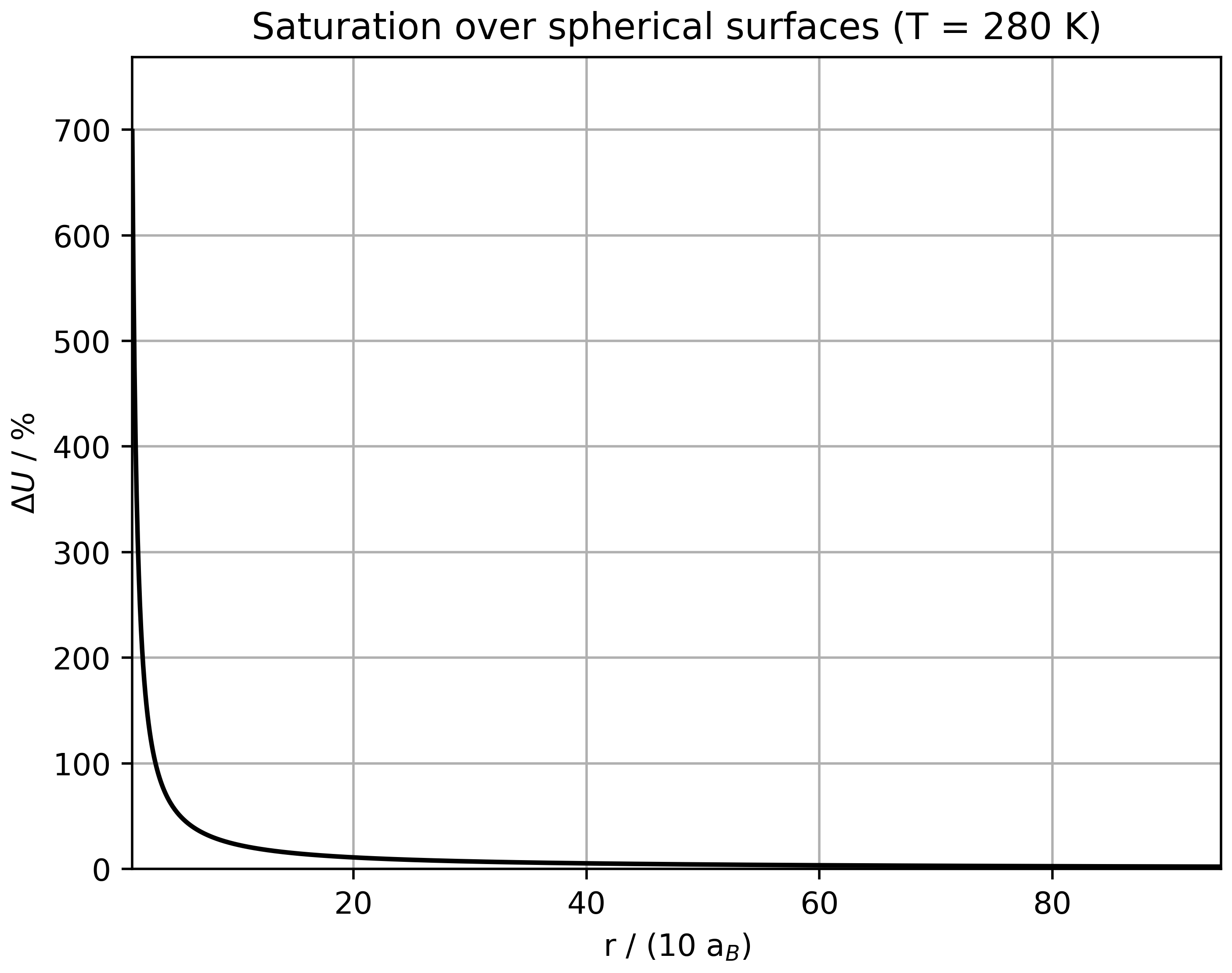
5.6 Photon gas

Imagine a cavity of temperature $T$ in equilibrium with electromagnetic radiation. We are looking for the spectral energy density $u\left(\omega\right)$ in the cavity. The properties of electromagnetic waves were discussed in Sect. 3.3. These are transverse waves. If the wave vector points in the z direction, $\mathbf {k} = k\mathbf {e}_z$, this follows for the electric field in the case of standing waves

\[ \begin{align} \mathbf{E}\left(z, t\right) = \left(E_{0, x}\mathbf{e}_x + E_{0, y}\mathbf{e}_y\right)\sin\left(kz\right)\sin\left(\omega t\right). \end{align} \]

Any phases were neglected. The B field can be determined from this. The cavity is cubic with volume $V = L^3$, and the walls are metallic. In this case, the parallel component of the electric field disappears at the surface, otherwise currents would be excited and energy would be dissipated. From this follow the discrete k-values

\[ \begin{align} k_iL = i\pi\Leftrightarrow k_i = \frac{\pi}{L}i \end{align} \]

with $i\in \mathbb{N}$ and $i\geq 1$, negative values ​​of $i$ must be neglected because this does not result in new solutions. Sums over $k_i$ values ​​can again be replaced by integrals:

\[ \begin{align} \sum_{k_i}^{}\dotsc = \frac{L}{\pi}\int_0^\infty\dotsc dk = \frac{L}{2\pi}\int_{-\infty}^{\infty}\dotsc dk. \end{align} \]

For a sum over all modes in the cavity applies

\[ \begin{align} \sum_{m = 1}^{2}\sum_{\mathbf{k}}^{}\dotsc = 2\sum_{\mathbf{k}}^{}\dotsc = 2\left(\frac{L}{2\pi}\right)^3\int\dotsc d^3k = \frac{2V}{\left(2\pi\right)^3}\int\dotsc d^3k. \end{align} \]

$m$ runs over the two possible polarization directions. For the energies $E = E\left(\mathbf{k}, m\right)$, according to Eq. (4.6)

\[ \begin{align} E\left(\mathbf{k}, m\right) = \hbar\omega\left(k\right) = \hbar ck. \end{align} \]

A microstate $r$ of the system is given by the population numbers

\[ \begin{align} r = \left(n_{\mathbf{k}, m}\right) \end{align} \]

given, i.e. the number of excitations for each vibration mode, one excitation is one photon. The energy of the microstate is $E_r\left(V\right)$

\[ \begin{align} E_r\left(V\right) = \sum_{m, \mathbf{k}}^{}\hbar\omega\left(k\right)n_{\mathbf{k}, m} = \hbar c\sum_{\mathbf{k}, m}^{}kn_{\mathbf{k}, m}. \end{align} \]

Now the average occupation numbers $\newoverline{n}_{\mathbf {k}, m}$ have to be determined. For this we start from the grand canonical partition function of a system without a polarization degree of freedom, i.e. $m = 1$:

\[ \begin{align} Y &= \sum_r\exp\left[-\beta\left(E_r - \mu N_r\right)\right] = \sum_{n_{\mathbf{p}_1 = 0}}^{\infty}\exp\left[-\beta\left(E_{p_1} - \mu\right)n_{\mathbf{p}_1}\right]\cdot\sum_{n_{\mathbf{p}_2} = 0}^{\infty}\exp\left[-\beta\left(E_{p_2} - \mu\right)n_{\mathbf{p}_2}\right]\cdot\dotsc\nonumber\\ &\stackrel{\href{ch-39-derivations-of-some-mathematical-formula.html#eq:geometr_reihe}{\text{Glg. (A.8)}}}{=} \prod_{\mathbf{p}}^{}\frac{1}{1 - \exp\left(-\beta\left(E_p - \mu\right)\right)}. \end{align} \]

It follows

\[ \begin{align} \newoverline{n}_{\mathbf{p}_i} &= \frac{1}{Y}\sum_rn_{\mathbf{p}_i}\exp\left[-\beta\left(E_r - \mu N_r\right)\right] = \frac{1}{Y}\sum_{n_{\mathbf{p}_1} = 0}^{\infty}\dotsc\sum_{n_{\mathbf{p}_i} = 0}^{\infty}\dotsc n_{\mathbf{p}_i}\exp\left[-\beta\left(E_{\mathbf{p}_i} - \mu\right)n_{\mathbf{p}_i}\right]\dotsc\nonumber\\ &= \frac{1}{Y}\sum_{n_{\mathbf{p}_1} = 0}^{\infty}\dotsc\left(\frac{1}{\beta}\frac{\partial}{\partial\mu}\sum_{n_{\mathbf{p}_i} = 0}^{\infty}\exp\left[-\beta\left(E_{\mathbf{p}_i} - \mu\right)n_{\mathbf{p}_i}\right]\right)\dotsc = \frac{1}{Y}\sum_{n_{\mathbf{p}_1} = 0}^{\infty}\dotsc\left(\frac{1}{\beta}\frac{\partial}{\partial\mu}\frac{1}{1 - \exp\left[-\beta\left(E_{\mathbf{p}_i} - \mu\right)\right]}\right)\dotsc\nonumber\\ &= \frac{1}{Y}\sum_{n_{\mathbf{p}_1} = 0}^{\infty}\dotsc\left(\frac{\exp\left[-\beta\left(E_{\mathbf{p}_i} - \mu\right)\right]}{\left(1 - \exp\left[-\beta\left(E_{\mathbf{p}_i} - \mu\right)\right]\right)^2}\right)\dotsc = \frac{\exp\left[-\beta\left(E_{\mathbf{p}_i} - \mu\right)\right]}{1 - \exp\left[-\beta\left(E_{\mathbf{p}_i} - \mu\right)\right]}. \end{align} \]

This is the Bose distribution, it applies to particles with integer spin:

The energy eigenvalues ​​$E_r\left(V\right)$ do not depend on the number of phonons $N$, so the following applies

\[ \begin{align} \mu = \newoverline{\frac{\partial E_r\left(V\right)}{\partial N}} = 0, \end{align} \]

the chemical potential disappears. Therefore applies

\[ \begin{align} \newoverline{n}_{\mathbf{k}, m} = \frac{1}{\exp\left(\beta E_k\right) - 1}. \end{align} \]

It follows

\[ \begin{align} E\left(T, V\right) = \newoverline{E_r\left(T, V\right)} &= \sum_{m, \mathbf{k}}^{}E_k\newoverline{n_k} = \frac{2V}{\left(2\pi\right)^3}\int\frac{\hbar ck}{\exp\left(\beta\hbar ck\right) - 1}d^3k = \frac{2V}{\left(2\pi\right)^3}4\pi\int_{0}^{\infty}\frac{\hbar ck^3}{\exp\left(\beta\hbar ck\right) - 1}dk\nonumber\\ &= V\int_{0}^{\infty}\underbrace{\frac{\hbar}{c^3\pi^2}\frac{\omega^3}{\exp\left(\beta\hbar\omega\right) - 1}}_{ = u\left(\omega\right)}d\omega. \end{align} \]

This is the Planck's radiation law. The ideas in this section are very specific, but Planck's distribution always applies when matter of temperature $T$ is in equilibrium with electromagnetic radiation. This equilibrium can always be assumed due to the high speed of the waves (speed of light). However, there may be deviations in the spectrum, such as absorption lines. Within a cavity in thermal equilibrium, the radiation is isotropic, so the spectral radiance applies

\[ \begin{align} J\left(\omega\right) = \frac{u\left(\omega\right)}{4\pi}c = \frac{\hbar}{4\pi^3c^2}\frac{\omega^3}{\exp\left(\frac{\hbar\omega}{k_BT}\right) - 1}. \end{align} \]

The spectral intensity $I\left(\omega\right)$ of a radiating surface is calculated from this:

\[ \begin{align} I\left(\omega\right) &= \int_{\vartheta = 0}^{\pi/2}\int_{\phi = 0}^{2\pi}J\left(\omega\right)\cos\left(\vartheta\right)\sin\left(\vartheta\right)d\vartheta d\phi = 2\pi\frac{1}{2}J\left(\omega\right) = \frac{\hbar}{4\pi^2c^2}\frac{\omega^3}{\exp\left(\frac{\hbar\omega}{k_BT}\right) - 1}. \end{align} \]

If you integrate this over the entire spectrum, the radiated power density follows

\[ \begin{align} \frac{P}{A} = \int_{0}^{\infty}I\left(\omega\right)d\omega = \frac{\hbar}{4\pi^2c^2}\int_{0}^{\infty}\frac{\omega^3}{\exp\left(\frac{\hbar\omega}{k_BT}\right) - 1}d\omega = \frac{k_B^4T^4}{4\pi^2c^2\hbar^3}\int_{0}^{\infty}\frac{x^3}{e^x - 1}d^x \end{align} \]

With Eq. (A.99) follows

\[ \begin{align} P = P\left(T\right) = \frac{k_B^4\pi^2}{60c^2\hbar^3}T^4.\tag{5.320}\label{eq:stefan-boltzmann} \end{align} \]

This is the Stefan-Boltzmann law, is defined

\[ \begin{align} \sigma \coloneqq\frac{k_B^4\pi^2}{60c^2\hbar^3} \end{align} \]

as the Stefan-Boltzmann constant. Real bodies emit at a temperature $T$ in the direction specified by $\vartheta$ and $\varphi$ at an angular frequency $\omega$ a factor of $J\left(\omega, T\right)$

\[ \begin{align} \epsilon = \epsilon\left(\omega, T, \vartheta, \varphi\right) \end{align} \]

different spectral radiance:

\[ \begin{align} J_{\text{real}}\left(\omega, T, \vartheta, \varphi\right) = \epsilon\left(\omega, T, \vartheta, \varphi\right)J\left(\omega, T\right). \end{align} \]

The factor $\epsilon$ is called emissivity. Imagine a small area $dA$ on the inner surface of the cavity. This area absorbs a power density

\[ \begin{align} \frac{dP_{\text{abs}}}{dA} = \int_{\omega = 0}^\infty\int_{\vartheta = 0}^{\pi/2}\int_{\varphi = 0}^{2\pi}\alpha\left(\omega, T, \vartheta, \varphi\right)J\left(\omega, T\right)\cos\left(\vartheta\right)\sin\left(\vartheta\right)d\varphi d\vartheta d\omega, \end{align} \]

Here the absorption coefficient $\alpha\left(\omega, T, \vartheta, \varphi\right)$ was introduced. Since a thermodynamic equilibrium is assumed, the emitted power density applies

\[ \begin{align} \frac{dP_{\text{emt}}}{dA} = \int_{\omega = 0}^\infty\int_{\vartheta = 0}^{\pi/2}\int_{\varphi = 0}^{2\pi}\epsilon\left(\omega, T, \vartheta, \varphi\right)J\left(\omega, T\right)\cos\left(\vartheta\right)\sin\left(\vartheta\right)d\varphi d\vartheta d\omega = \frac{dP_{\text{abs}}}{dA}. \end{align} \]

It follows

\[ \begin{align} \int_{\omega = 0}^\infty\int_{\vartheta = 0}^{\pi/2}\int_{\varphi = 0}^{2\pi}\left(\epsilon\left(\omega, T, \vartheta, \varphi\right) - \alpha\left(\omega, T, \vartheta, \varphi\right)\right)J\left(\omega, T\right)\cos\left(\vartheta\right)\sin\left(\vartheta\right)d\varphi d\vartheta d\omega = 0. \end{align} \]

Since the spectral energy density of the cavity is constant, even

\[ \begin{align} \int_{\vartheta = 0}^{\pi/2}\int_{\varphi = 0}^{2\pi}\left[\epsilon\left(\omega, T, \vartheta, \varphi\right) - \alpha\left(\omega, T, \vartheta, \varphi\right)\right]\sin\left(\vartheta\right)\cos\left(\vartheta\right)d\varphi d\vartheta = 0. \end{align} \]

You define it

\[ \begin{align} \epsilon\left(\omega, T\right) \coloneqq\int_{\vartheta = 0}^{\pi/2}\int_{\varphi = 0}^{2\pi}\epsilon\left(\omega, T, \vartheta, \varphi\right)\sin\left(\vartheta\right)\cos\left(\vartheta\right)d\varphi d\vartheta. \end{align} \]

and analogously for the absorption coefficient, follows

\[ \begin{align} \epsilon\left(\omega, T\right) = \alpha\left(\omega, T\right). \end{align} \]

Now we look specifically at the direction given by $\vartheta$ and $\varphi$. Here $dA$ is the spectral radiance

\[ \begin{align} & J_\text{out}\left(\omega, T\right) = J\left(\omega, T\right)\nonumber\\ &= J\left(\omega, T\right)\left(\epsilon\left(\omega, T, \vartheta, \varphi\right) + \int_{\varphi' = 0}^{2\pi}\int_{\vartheta' = 0}^{\pi/2}s\left(\vartheta', \varphi', \vartheta, \varphi, \omega, T\right)\cos\left(\vartheta'\right)\sin\left(\vartheta'\right)d\vartheta'd\varphi'\right) \end{align} \]

out of. The expression in brackets results in one. The scattering cross section $s\left(\vartheta', \varphi', \vartheta, \varphi, \omega, T\right)$ was defined. It describes the extent to which radiation incident from the direction $\left(\vartheta', \varphi'\right)$ is redirected in the direction $\left(\vartheta, \varphi\right)$ without being absorbed and re-emitted in between. The following applies to the incident spectral radiance

\[ \begin{align} & J_\text{in}\left(\omega, T\right) = J\left(\omega, T\right)\nonumber\\ &= J\left(\omega, T\right)\left(\alpha\left(\omega, T, \vartheta, \varphi\right) + \int_{\varphi' = 0}^{2\pi}\int_{\vartheta' = 0}^{\pi/2}s\left(\vartheta, \varphi, \vartheta', \varphi', \omega, T\right)\cos\left(\vartheta'\right)\sin\left(\vartheta'\right)d\vartheta'd\varphi'\right) \end{align} \]

The expression in brackets must return to one. Since the Maxwell equations, like the Schrödinger equation, are invariant against time reversal, the following applies

\[ \begin{align} s\left(\vartheta, \varphi, \vartheta', \varphi', \omega, T\right) = s\left(\vartheta', \varphi', \vartheta, \varphi, \omega, T\right). \end{align} \]

It follows

\[ \begin{align} \epsilon\left(\omega, T, \vartheta, \varphi\right) = \alpha\left(\omega, T, \vartheta, \varphi\right) \end{align} \]

This is called Kirchhoff's radiation law. Since a body can never absorb more than the radiation that hits it, $\alpha\leq1$ applies, so it follows

\[ \begin{align} \epsilon\leq1. \end{align} \]

Bodies with $\epsilon\left(\vartheta, \varphi, \omega\right) = 1$ are called black bodies, so the Stefan-Boltzmann law only applies to black bodies.