2 Classic mechanics
Classical mechanics deals with mass points, i.e. masses without spatial extension, which move at speeds $\ll c$ (transition to relativity theory) and are not too light (transition to quantum mechanics).
2.1 Newtonian mechanics
Classical mechanics is based on Newton's axioms [18]. The most important axiom is Newton's Second Axiom:
Let a point mass $m$ with momentum $\mathbf{p}$ be given, on which the force $\mathbf{F}$ acts, then the following applies
\[ \begin{align} \frac{d\mathbf{p}}{dt} = \mathbf{F}.\tag{2.1}\label{eq:newton_II} \end{align} \]
The impulse is defined by
\[ \begin{align} \mathbf{p} \coloneqq m\frac{d\mathbf{r}}{dt}, \end{align} \]
where $\mathbf{r} = \mathbf{r}\left(t\right)$ is the trajectory of the mass point. The First Axiom is a special case of the Second and is therefore insignificant. Newton's Third Axiom is:
Let two masses $m_1$ and $m_2$ be given. Let $\mathbf{F}_1$ and $\mathbf{F}_2$ be the forces on the masses due to the pairwise interaction (WW). Then applies
\[ \begin{align} \mathbf{F}_1 = -\mathbf{F}_2. \end{align} \]
To complete the theory, two additions to Newton's axioms are introduced. First, one determines that if $N \geq 1$ forces $\mathbf{F}_j$ act on a mass point, in Eq. (2.1) to use the sum of these forces is:
\[ \begin{align} m\frac{d^2\mathbf{r}}{dt^2} = \sum_{j = 1}^{N}\mathbf{F}_j \end{align} \]
Furthermore, it is assumed that the force $\mathbf{F}_1$ is parallel to the connecting line $\mathbf{r}_1 - \mathbf{r}_2$:
\[ \begin{align} \mathbf{F}_1 \parallel \mathbf{r}_1 - \mathbf{r}_2 \end{align} \]
Let two point masses $m_1, m_2$ be given at the locations $\mathbf{r}_1, \mathbf{r}_2$. One defines the center of gravity $\mathbf{R}$ by
\[ \begin{align} \mathbf{R} \coloneqq \frac{m_1\mathbf{r}_1 + m_2\mathbf{r}_2}{M} \end{align} \]
with the total mass
\[ \begin{align} M \coloneqq m_1 + m_2. \end{align} \]
Newton's Second Axiom applies to the acceleration of the center of gravity
\[ \begin{align} \frac{d^2\mathbf{R}}{dt^2} = \frac{m_1\frac{d^2\mathbf{r}_1}{dt^2} + m_2\frac{d^2\mathbf{r}_2}{dt^2}}{M} = \frac{1}{M}\left(\mathbf{F}_1 + \mathbf{F}_2\right), \end{align} \]
where $\mathbf{F}_1$ represents the total force acting on $m_1$ and $\mathbf{F}_2$ represents the total force acting on $m_2$. These can be divided into an internal and an external force:
\[ \begin{align} \mathbf{F}_1 &= \mathbf{F}_1^{\text{(int)}} + \mathbf{F}_1^{\text{(ext)}}, & {} & \mathbf{F}_2 = \mathbf{F}_2^{\text{(int)}} + \mathbf{F}_2^{\text{(ext)}} \end{align} \]
The internal force arises from interactions within the system. Due to Newton's third axiom,
\[ \begin{align} \mathbf{F}_1^{\text{(int)}} = -\mathbf{F}_2^{\text{(int)}}. \end{align} \]
So you get
\[ \begin{align} \frac{d^2\mathbf{R}}{dt^2} = \frac{1}{M}\left(\mathbf{F}_1^{\text{(ext)}} + \mathbf{F}_2^{\text{(ext)}}\right). \end{align} \]
So a kind of Newton's second axiom applies
\[ \begin{align} M\frac{d^2\mathbf{R}}{dt^2} = \sum_{i}^{}\mathbf{F}_i^{\text{(ext)}} \end{align} \]
for the movement of the center of gravity coordinate. The relative coordinate is carried out in the same way
\[ \begin{align} \mathbf{r} \coloneqq \mathbf{r}_2 - \mathbf{r}_1 \end{align} \]
a. This satisfies the equation of motion
\[ \begin{align} \frac{d^2\mathbf{r}}{dt^2} = \frac{d^2\mathbf{r}_2}{dt^2} - \frac{d^2\mathbf{r}_1}{dt^2} = \frac{\mathbf{F}_1}{m_1} - \frac{\mathbf{F}_2}{m_2}\Leftrightarrow \frac{m_1m_2}{m_1 + m_2}\frac{d^2\mathbf{r}}{dt^2} = \frac{m_2}{m_1 + m_2}\mathbf{F}_1 - \frac{m_1}{m_1 + m_2}\mathbf{F}_2. \end{align} \]
If you now only assume internal WW, you get
\[ \begin{align} \mu\frac{d^2\mathbf{r}}{dt^2} = \mathbf{F}_1^{\text{(int)}}. \end{align} \]
This was the reduced mass
\[ \begin{align} \mu \coloneqq \frac{m_1m_2}{M} \end{align} \]
introduced. With vanishing external forces, a mass $\mu$ effectively moves in the force field of the pairwise WW, its position vector is $\mathbf{r}$. Some of the results also hold for $N\in \mathbb{N}$ with $N\geq 1$ particles. First you can get a total mass
\[ \begin{align} M \coloneqq \sum_{i = 1}^{N}m_i \end{align} \]
and a center of gravity coordinate
\[ \begin{align} \mathbf{R} \coloneqq \frac{\sum_{i = 1}^{N}m_i\mathbf{r}_i}{M} \end{align} \]
define. You derive this twice in time and get
\[ \begin{align} M\frac{d^2}{dt^2}\mathbf{R} = \sum_{i = 1}^{N}m_i\frac{d^2}{dt^2}\mathbf{r}_i = \sum_{i = 1}^{N}\mathbf{F}_i. \end{align} \]
It applies again
\[ \begin{align} \mathbf{F}_i = \mathbf{F}_i^{\text{(int)}} + \mathbf{F}_i^{\text{(ext)}} = \sum_{\substack{j = 1,\\j\not = i}}^{N}\mathbf{F}_i^{(j)} + \mathbf{F}_i^{\text{(ext)}}. \end{align} \]
Here $\mathbf{F}_i^{(j)}$ is the force that the $jth particle exerts on the $ith particle. Thus you get
\[ \begin{align} \sum_{i = 1}^{N}\mathbf{F}_i = \sum_{\substack{i, j = 1,\\i\not = j}}^{N}\mathbf{F}_i^{(j)} + \sum_{i = 1}^{N}\mathbf{F}_i^{\text{(ext)}} = \sum_{\substack{i, j = 1,\\i>j}}^{N}\mathbf{F}_i^{(j)} + \mathbf{F}_j^{(i)} + \sum_{i = 1}^{N}\mathbf{F}_i^{\text{(ext)}} = \sum_{\substack{i, j = 1,\\i>j}}^{N}\mathbf{F}_i^{(j)} - \mathbf{F}_i^{(j)} + \sum_{i = 1}^{N}\mathbf{F}_i^{\text{(ext)}} = \sum_{i = 1}^{N}\mathbf{F}_i^{\text{(ext)}}. \end{align} \]
This became Newton's third axiom
\[ \begin{align} \mathbf{F}_i^{(j)} = -\mathbf{F}_j^{(i)} \end{align} \]
used. This means: The internal WWs have no influence on the trajectory of the center of gravity. If no external forces act, the total momentum is constant; this is called law of conservation of momentum.
There is a formulation of Newtonian mechanics for rotations (rotational movements). The angular momentum $\mathbf{L}$ of a particle is defined by
\[ \begin{align} \mathbf{L} \coloneqq \mathbf{r}\times\mathbf{p}.\tag{2.23}\label{eq:def_angular_momentum} \end{align} \]
The torque $\mathbf{F}$ is defined as
\[ \begin{align} \mathbf{D} \coloneqq \mathbf{r}\times\mathbf{F}. \end{align} \]
By deriving Eq. (2.23) follows
\[ \begin{align} \frac{d}{dt}\mathbf{L} = \frac{d\mathbf{r}}{dt}\times\mathbf{p} + \mathbf{r}\times\frac{d\mathbf{p}}{dt} = \mathbf{r}\times\mathbf{F} = \mathbf{D}. \end{align} \]
This is also called Newton's Second Axiom of Rotation. For $N\in\mathbb{N}$ with $N\geq 1$ particles one obtains a total angular momentum of
\[ \begin{align} \mathbf{L} = \sum_{i = 1}^{N}\mathbf{L}_i = \sum_{i = 1}^{m}\mathbf{r}_i\times\mathbf{p}_i. \end{align} \]
This applies to this one
\[ \begin{align} \frac{d\mathbf{L}}{dt} &= \sum_{i = 1}^{N}\mathbf{r}_i\times\left(\mathbf{F}_i^{\text{(int)}} + \mathbf{F}_i^{\text{(ext)}}\right) = \sum_{\substack{i, j = 1,\\i\not = j}}^{N}\mathbf{r}_i\times\mathbf{F}_i^{(j)} + \sum_{i = 1}^{N}\mathbf{r}_i\times\mathbf{F}_i^{\text{(ext)}}\nonumber\\ &= \sum_{\substack{i, j = 1,\\i>j}}^{N}\mathbf{r}_i\times\mathbf{F}_i^{(j)} + \mathbf{r}_j\times\mathbf{F}_j^{(i)} + \sum_{i = 1}^{N}\mathbf{r}_i\times\mathbf{F}_i^{\text{(ext)}} = \sum_{\substack{i, j = 1,\\i>j}}^{N}\mathbf{F}_i^{(j)}\times\left(\mathbf{r}_i - \mathbf{r}_j\right) + \sum_{i = 1}^{N}\mathbf{r}_i\times\mathbf{F}_i^{\text{(ext)}}\nonumber\\ &= \sum_{i = 1}^{N}\mathbf{r}_i\times\mathbf{F}_i^{\text{(ext)}}. \end{align} \]
Newton's third axiom was used again as well as the additional statement that the force between two particles acts along the line connecting them. If no external forces act, the angular momentum is conserved; this is called law of conservation of angular momentum.
The concept of energy should be introduced. A force field is a function $\mathbf{F} = \mathbf{F}\left(\mathbf{r}\right)$, which assigns to each point $\mathbf{r}$ a force $\mathbf{F}\left(\mathbf{r}\right)$ acting there. A mass point moves along the trajectory $\mathbf{r} = \mathbf{r}\left(t\right)$. Then you define the work $W$ that the force field does at the mass point in the time interval $\left[t_1, t_2\right]$ by
\[ \begin{align} W \coloneqq \int_{t_1}^{t_2}\mathbf{F}\left(\mathbf{r}\left(t\right)\right)\cdot\frac{d\mathbf{r}}{dt}dt. \end{align} \]
Using Newton's Second Axiom and partial integration follows
\[ \begin{align} W = \int_{t_1}^{t_2}m\frac{d^2\mathbf{r}}{dt^2}\cdot\frac{d\mathbf{r}}{dt}dt &= \left[m\frac{d\mathbf{r}}{dt}\cdot\frac{d\mathbf{r}}{dt}\right]_{t_1}^{t_2} - \int_{t_1}^{t_2}m\frac{d\mathbf{r}}{dt}\cdot\frac{d^2\mathbf{r}}{dt^2}dt\nonumber\\ \Leftrightarrow W &= \frac{1}{2}m\mathbf{v}\left(t_2\right)^2 - \frac{1}{2}m\mathbf{v}\left(t_1\right)^2. \end{align} \]
Define the kinetic energy $E_{\text{kin}}$ by
\[ \begin{align} E_{\text{kin}} \coloneqq \frac{1}{2}m\mathbf{v}^2, \end{align} \]
follows
\[ \begin{align} W = \Delta E_{\text{kin}}. \end{align} \]
So the work done by the field becomes kinetic energy. Furthermore, a force field is called conservative, if a potential $U = U\left(\mathbf{r}\right)$ exists with
\[ \begin{align} \mathbf{F} = -\nabla U. \end{align} \]
In this case, according to Eq. (B.47)
\[ \begin{align} \nabla\times\mathbf{F} = \mathbf{0}, \end{align} \]
Thus, using Stokes' theorem, Eq. (15.26)
\[ \begin{align} \int_{\partial A}\mathbf{F}\cdot d\mathbf{s} = 0 \end{align} \]
for each surface $A$, so that the work done is independent of the path. Define the total energy of the particle by
\[ \begin{align} E \coloneqq E_{\text{kin}} + U, \end{align} \]
so this size is obtained:
\[ \begin{align} \frac{dE}{dt} &= \frac{dE_{\text{kin}}}{dt} + \frac{dU}{dt} = \frac{1}{2}m2\frac{d\mathbf{r}}{dt}\cdot\frac{d^2\mathbf{r}}{dt^2} + \nabla U\cdot\frac{d\mathbf{r}}{dt}\nonumber\\ &= \left(m\frac{d^2\mathbf{r}}{dt^2} + \nabla U\right)\cdot\frac{d\mathbf{r}}{dt} = \left(\mathbf{F} + \nabla U\right)\cdot\frac{d\mathbf{r}}{dt} = \left(-\nabla U + \nabla U\right)\cdot\frac{d\mathbf{r}}{dt} = 0 \end{align} \]
\[ \begin{align} \Rightarrow \frac{dE}{dt} = 0 \end{align} \]
The energy of a particle moving under the influence of a conservative force is therefore constant.
There are two other formulations of classical mechanics, the Lagrange formalism and the Hamilton formalism. Both can be derived from Newton's axioms.
2.2 Lagrange formalism
Newtonian mechanics is practical for flying points of mass (atoms in a gas, planets in a solar system) or rigid bodies (ships, airplanes). In principle, these can move freely in any direction. However, situations in which a mass point is restricted in its freedom of movement are common, for example a marble in a marble run, a billiard ball on a table or a train on a track. Such systems are subject to constraints. If the system consists of exactly one particle with the trajectory $\mathbf{r} = \mathbf{r}\left(t\right)$, then one can have a constraint in the form
\[ \begin{align} g\left(\mathbf{r}, t\right) = 0\tag{2.38}\label{eq:def_holonome_zwangsbedingung} \end{align} \]
write. $g$ is some scalar field. The condition $g = 0$ can be imagined as a surface. This surface can also be explicitly time-dependent, such as a vertically accelerated pool table. Eq. (2.38) is called holonomic constraint, all other constraints are called nonholonomic. This would be the case, for example, if $g$ were a function of $\frac{d\mathbf{r}}{dt}$. Explicitly time-dependent constraints are called rheonome, while time-independent constraints are called skleronome. In general you have $N$ particles, in this case you can set up $R$ constraints
\[ \begin{align} g_\alpha\left(\mathbf{r}_1, \dotsc, \mathbf{r}_N, t\right) = 0 \end{align} \]
with $1\leq\alpha\leq R$ and $R\leq 3N - 1$. At $R = 3N$ no movement could occur since each constraint eliminates one degree of freedom.
2.2.1 Lagrange equations 1st Art
Compliance with the constraint conditions is ensured by the so-called coercive forces. These are perpendicular to the surface specified by the constraint - this can easily be seen when moving on a table, for example. Although the friction force acts tangentially to the table, the friction force has nothing to do with compliance with the constraint and is therefore not a constraint. So you can use a constraint force $\mathbf{Z}$
\[ \begin{align} \mathbf{Z}\left(\mathbf{r}, t\right) = \lambda\left(t\right)\nabla g\left(\mathbf{r}, t\right). \end{align} \]
The multiplier $\lambda$ is time dependent because the forcing force depends on the time dependent trajectory. You can now write it down as an equation of motion
\[ \begin{align} m\frac{d^2}{dt^2}\mathbf{r} = \mathbf{F} + \lambda\left(t\right)\nabla g\left(\mathbf{r}, t\right), \end{align} \]
here $\mathbf{F}$ is the sum of all non-constraint forces (gravity, friction force, etc.). If you have given two constraints, you can generalize this to:
\[ \begin{align} m\frac{d^2}{dt^2}\mathbf{r} = \mathbf{F} + \sum_{\alpha = 1}^{2}\lambda_\alpha\left(t\right)\nabla g_\alpha\left(\mathbf{r}, t\right). \end{align} \]
This is plausible: $g_1 = 0$ and $g_2 = 0$ define two areas in which the trajectory runs. $\nabla g_1$ and $\nabla g_2$ are each perpendicular to the corresponding surface and thus also to the trajectory, and they are also linearly independent. Therefore $\sum_{\alpha = 1}^{2}\lambda_\alpha\left(t\right)\nabla g_\alpha\left(\mathbf{r}, t\right)$ is a general approach for a force perpendicular to the trajectory, i.e. for a general forcing force. Together with $g_1\left(\mathbf{r}, t\right) = g_2\left(\mathbf{r}, t\right) = 0$ you now have five equations for the five unknown functions $x\left(t\right), y\left(t\right), z\left(t\right), \lambda_1\left(t\right), \lambda_2\left(t\right)$. So there is a chance of solvability. In general, one has given $N$ particles with the Cartesian coordinates $x_n$ with $1\leq n\leq 3N$, here $x_1, x_2, x_3$ are the coordinates of the first particle $x_4, x_5, x_6$ are those of the second, etc. If one has $R\leq 3N - 1$ holonomic constraints $g_j\left(\mathbf{r}, t\right) = 0$ can be written down as equations of motion
\[ \begin{align} m_n\frac{d^2x_n}{dt^2} = F_n + \sum_{\alpha = 1}^{R}\lambda_\alpha\left(t\right)\frac{\partial g_\alpha\left(x_1, \dotsc, x_{3N}, t\right)}{\partial x_n}.\tag{2.43}\label{eq:lagrange_first_art} \end{align} \]
Here, $m_1 = m_2 = m_3$ is the mass of the first particle, etc. Together with the constraints, you get $3N + R$ equations for the $3N + R$ functions $x_n\left(t\right), \lambda_\alpha\left(t\right)$. These $3N + R$ equations are called Lagrange equations of the first kind.
2.2.2 Lagrange equations 2nd kind
If you are not interested in calculating the forcing forces, eliminating them is a good idea. This is now being done.
As noted, each of the constraints $g_\alpha$ eliminates one degree of freedom. The number of degrees of freedom
\[ \begin{align} f = 3N - R \end{align} \]
here is the number of numbers necessary to determine the location of all $N$ particles. These numbers are called generalized coordinates $q_1, \dotsc, q_f$. You must meet two conditions:
- You need to set the Cartesian coordinates, $x_n = x_n\left(q_1, \dotsc, q_f, t\right)$ for all $1\leq n\leq 3N$.
- You have to consider the constraints: $g_\alpha\left(q_1, \dotsc, q_f, t\right) = 0$ for $1\leq\alpha\leq R$ and all possible $q_i$.
The second condition can be expressed formally as:
\[ \begin{align} \frac{dg_\alpha}{dq_k} = \sum_{n = 1}^{3N}\frac{\partial g_\alpha}{\partial x_n}\frac{\partial x_n}{\partial q_k} = 0. \end{align} \]
If you multiply Eq. (2.43) with $\frac{\partial x_n}{\partial q_k}$, one obtains
\[ \begin{align} m_n\frac{d^2x_n}{dt^2}\frac{\partial x_n}{\partial q_k} = F_n\frac{\partial x_n}{\partial q_k} + \sum_{\alpha = 1}^{R}\lambda_\alpha\left(t\right)\frac{\partial g_\alpha\left(x_1, \dotsc, x_{3N}, t\right)}{\partial x_n}\frac{\partial x_n}{\partial q_k}. \end{align} \]
If you sum this over $n$, it follows
\[ \begin{align} \sum_{n = 1}^{3N}m_n\frac{d^2x_n}{dt^2}\frac{\partial x_n}{\partial q_k} = \sum_{n = 1}^{3N}F_n\frac{\partial x_n}{\partial q_k}.\tag{2.47}\label{eq:lagrange_deriv_3} \end{align} \]
This equation applies to all $1\leq k\leq f$. Coercive forces no longer appear here. The following notations are introduced:
\[ \begin{align} x \coloneqq \left(x_1, \dotsc, x_n\right), & {} & \newdot{x} \coloneqq \left(\newdot{x}_1, \dotsc, \newdot{x}_n\right)\\ q \coloneqq \left(q_1, \dotsc, q_n\right), & {} & \newdot{q} \coloneqq \left(\newdot{q}_1, \dotsc, \newdot{q}_n\right) \end{align} \]
The $\newdot{q}_i$ is also referred to as generalized velocities. You now derive the transformation equation
\[ \begin{align} x_n = x_n\left(q, t\right) \end{align} \]
totally after the time:
\[ \begin{align} \newdot{x}_n = \frac{d}{dt}x_n\left(q, t\right) = \sum_{k = 1}^{f}\frac{\partial x_n}{\partial q_k}\newdot{q}_k + \frac{\partial x_n}{\partial t} = \newdot{x}_n\left(q, \newdot{q}, t\right)\tag{2.51}\label{eq:transformation_lagrange_geschwindigkeiten} \end{align} \]
It follows
\[ \begin{align} \frac{\partial\newdot{x}_n}{\partial\newdot{q}_k} = \frac{\partial x_n}{\partial q_k}. \end{align} \]
For the kinetic energy $T$ applies
\[ \begin{align} T = T\left(\newdot{x}\right) = \sum_{n = 1}^{3N}\frac{1}{2}m_n\newdot{x}_n^2.\tag{2.53}\label{eq:newton_kinetische_energie} \end{align} \]
Here you set Eq. (2.51) on:
\[ \begin{align} T = T\left(q, \newdot{q}, t\right) = \sum_{i, k = 1}^{f}m_{i, k}\left(q, t\right)\newdot{q}_i\newdot{q}_k + \sum_{k = 1}^{f}b_k\left(q, t\right)\newdot{q}_k + c\left(q, t\right) \end{align} \]
From Eq. (2.53) follows
\[ \begin{align} \frac{\partial T\left(q, \newdot{q}, t\right)}{\partial q_k} = \sum_{n = 1}^{3N}m_n\newdot{x}_n\frac{\partial\newdot{x}_n}{\partial q_k}.\tag{2.55}\label{eq:lagrange_deriv_2} \end{align} \]
Still applies
\[ \begin{align} \frac{\partial T\left(q, \newdot{q}, t\right)}{\partial\newdot{q}_k} = \sum_{n = 1}^{3N}m_n\newdot{x}_n\frac{\partial\newdot{x}_n}{\partial\newdot{q}_k} = \sum_{n = 1}^{3N}m_n\newdot{x}_n\frac{\partial x_n}{\partial q_k}. \end{align} \]
If you derive this totally according to time, you get
\[ \begin{align} \frac{d}{dt}\frac{\partial T}{\partial\newdot{q}_k} = \sum_{n = 1}^{3N}m_n\frac{d^2x_n}{dt^2}\frac{\partial x_n}{\partial q_k} + \sum_{n = 1}^{3N}m_n\newdot{x}_n\frac{\partial\newdot{x}_n}{\partial q_k}.\tag{2.57}\label{eq:lagrange_deriv_1} \end{align} \]
In the last term the following identity was exploited:
\[ \begin{align} \frac{d}{dt}\frac{\partial x_n}{\partial q_k} = \sum_{l = 1}^{f}\frac{\partial^2x_n}{\partial q_l\partial q_k}\newdot{q}_l + \frac{\partial^2 x_n}{\partial t\partial q_k} = \frac{\partial}{\partial q_k}\left(\sum_{l = 1}^{f}\frac{\partial x_n}{\partial q_l}\newdot{ q_l} + \frac{\partial x_n}{\partial t}\right) = \frac{\partial}{\partial q_k}\frac{dx_n}{dt} \end{align} \]
One now defines generalized forces:
\[ \begin{align} Q_k \coloneqq \sum_{n = 1}^{3N}F_n\frac{\partial x_n}{\partial q_k} \end{align} \]
This definition is combined with Eq. (2.57) and Eq. (2.55) in Eq. (2.47):
\[ \begin{align} \sum_{n = 1}^{3N}m_n\frac{d^2x_n}{dt^2}\frac{\partial x_n}{\partial q_k} = \sum_{n = 1}^{3N}F_n\frac{\partial x_n}{\partial q_k} & {} & \Leftrightarrow \sum_{n = 1}^{3N}m_n\frac{d^2x_n}{dt^2}\frac{\partial x_n}{\partial q_k} = Q_k\nonumber\\ \Leftrightarrow\frac{d}{dt}\frac{\partial T}{\partial\newdot{q}_k} - \sum_{n = 1}^{3N}m_n\newdot{x}_n\frac{\partial\newdot{x}_n}{\partial q_k} = Q_k & {} & \Leftrightarrow \frac{d}{dt}\frac{\partial T}{\partial\newdot{q}_k} - \frac{\partial T}{\partial q_k} = Q_k \end{align} \]
You bet on your strengths
\[ \begin{align} F_n = -\frac{\partial U\left(x, \newdot{x}, t\right)}{\partial x_n} + \frac{d}{dt}\frac{\partial U\left(x, \newdot{x}, t\right)}{\partial\newdot{x}_n}\tag{2.61}\label{eq:lagrange_kraefte} \end{align} \]
with a potential $U = U\left(x, \newdot{x}, t\right)$. In the case of a speed-independent conservative force, this reduces to the form known from Newtonian mechanics, the second term has been added to take the speed dependence into account. $\left(x, \newdot{x}\right)$ can be bijectively mapped to $\left(q, \newdot{q}\right)$, so you can note it down
\[ \begin{align} U = U\left(q, \newdot{q}, t\right). \end{align} \]
Now you can write
\[ \begin{align} Q_k = \sum_{n = 1}^{3N}F_n\frac{\partial x_n}{\partial q_k} = -\sum_{n = 1}^{3N}\frac{\partial U}{\partial x_n}\frac{\partial x_n}{\partial q_k} + \frac{d}{dt}\sum_{n = 1}^{3N}\frac{\partial U}{\partial\newdot{x}_n}\frac{\partial x_n}{\partial q_k} = -\frac{\partial U}{\partial q_k} + \frac{d}{dt}\frac{\partial U}{\partial\newdot{q}_k}. \end{align} \]
The equation follows
\[ \begin{align} \frac{d}{dt}\frac{\partial\left(T - U\right)}{\partial\newdot{q}_k} = \frac{\partial\left(T - U\right)}{\partial q_k}. \end{align} \]
One defines the Lagrange function $L$ by
\[ \begin{align} L\left(q, \newdot{q}, t\right) \coloneqq T\left(q, \newdot{q}, t\right) - U\left(q, \newdot{q}, t\right). \end{align} \]
This gives you
\[ \begin{align} \frac{d}{dt}\frac{\partial L\left(q, \newdot{q}, t\right)}{\partial\newdot{q}_k} = \frac{\partial L\left(q, \newdot{q}, t\right)}{\partial q_k}. \end{align} \]
For $1\leq k\leq f$ these are the Lagrange equations of the second kind.
2.3 Hamilton formalism
First define the canonical impulses by
\[ \begin{align} p_i \coloneqq\frac{\partial L}{\partial\newdot{q}_i} \end{align} \]
for $1\leq i\leq f$. One now eliminates the generalized velocities $\newdot{q}$:
\[ \begin{align} p_i = \frac{\partial L\left(q, \newdot{q}, t\right)}{\partial\newdot{q}_i}\to\newdot{q}_j = \newdot{q}_j\left(q, p, t\right) \end{align} \]
The Hamilton function $H$ is defined by
\[ \begin{align} H\left(q, p, t\right) \coloneqq \sum_{i = 1}^{f}\newdot{q}_i\left(q, p, t\right)p_i - L\left(q, \newdot{q}\left(q, p, t\right), t\right). \end{align} \]
The Hamilton's equations or also canonical equations follow by partial differentiation:
\[ \begin{align} \frac{\partial H}{\partial q_k} &= \sum_{i = 1}^{f}\frac{\partial\newdot{q}_i}{\partial q_k}p_i - \frac{\partial L}{\partial q_k} - \sum_{i = 1}^{f}\frac{\partial L}{\partial\newdot{q}_i}\frac{\partial\newdot{q}_i}{\partial q_k} = -\frac{\partial L}{\partial q_k} = -\frac{d}{dt}\left(\frac{\partial L}{\partial\newdot{q}_k}\right) = -\newdot{p}_k\tag{2.70}\label{eq:hamilton_0}\\ \frac{\partial H}{\partial p_k} &= \sum_{i = 1}^{f}\frac{\partial\newdot{q}_i}{\partial p_k}p_i + \newdot{q}_k - \sum_{i = 1}^{f}\frac{\partial L}{\partial\newdot{q}_i}\frac{\partial\newdot{q}_i}{\partial p_k} = \newdot{q}_k\tag{2.71}\label{eq:hamilton_1}\\ \frac{\partial H}{\partial t} &= \sum_{i = 1}^{f}\frac{\partial\newdot{q}_i}{\partial t}p_i - \sum_{i = 1}^{f}\frac{\partial L}{\partial\newdot{q}_i}\frac{\partial\newdot{q}_i}{\partial t} - \frac{\partial L}{\partial t} = -\frac{\partial L}{\partial t}\tag{2.72}\label{eq:hamilton_2} \end{align} \]
The space of $\left(q, p\right)$ is called phase space.
2.3.1 Poisson bracket
Any two quantities $F$, $K$ can only depend on $\left(q, p, t\right)$. One defines the Poisson bracket $\left\lbrace F, K\right\rbrace$ of $F$ and $K$ by
\[ \begin{align} \left\lbrace F, K\right\rbrace \coloneqq \sum_{i = 1}^f\left(\frac{\partial F}{\partial q_i}\frac{\partial K}{\partial p_i} - \frac{\partial F}{\partial p_i}\frac{\partial K}{\partial q_i}\right).\tag{2.73}\label{eq:poisson_bracket_def} \end{align} \]
The following are immediate consequences:
\[ \begin{align} \left\lbrace F + G, K\right\rbrace &= \left\lbrace F, K\right\rbrace + \left\lbrace G, K\right\rbrace,\tag{2.74}\label{eq:poisson_bracket_prop_1}\\ \left\lbrace F, K\right\rbrace &= -\left\lbrace K, F\right\rbrace,\tag{2.75}\label{eq:poisson_bracket_prop_2}\\ \left\lbrace F, F\right\rbrace &= 0.\tag{2.76}\label{eq:poisson_bracket_prop_3} \end{align} \]
Apply in the Hamilton formalism
\[ \begin{align} \frac{\partial q_i}{\partial q_j} = \delta_{i, j}, & {} & \frac{\partial q_i}{\partial p_j} = 0, & {} & \frac{\partial q_i}{\partial t} = 0,\\ \frac{\partial p_i}{\partial q_j} = 0, & {} & \frac{\partial p_i}{\partial p_j} = \delta_{i, j}, & {} & \frac{\partial p_i}{\partial t} = 0. \end{align} \]
Furthermore are
\[ \begin{align} \left\lbrace F, q_j\right\rbrace = -\frac{\partial F}{\partial p_j}, & {} & \left\lbrace F, p_j\right\rbrace = \frac{\partial F}{\partial q_j}. \end{align} \]
This follows further
\[ \begin{align} \left\lbrace q_i, q_j\right\rbrace = 0, & {} & \left\lbrace p_i, p_j\right\rbrace = 0, & {} & \left\lbrace p_i, q_j\right\rbrace = -\delta_{i, j}. \end{align} \]
For the total time derivative of $F$ we now get
\[ \begin{align} \frac{dF}{dt} = \sum_{i = 1}^f\frac{\partial F}{\partial q_i}\newdot{q}_i + \sum_{i = 1}^f\frac{\partial F}{\partial p_i}\newdot{p}_i + \frac{\partial F}{\partial t} = \sum_{i = 1}^f\frac{\partial F}{\partial q_i}\frac{\partial H}{\partial p_i} - \sum_{i = 1}^f\frac{\partial F}{\partial p_i}\frac{\partial H}{\partial q_i} + \frac{\partial F}{\partial t} \end{align} \]
\[ \begin{align} \Leftrightarrow \frac{dF}{dt} = \left\lbrace F, H\right\rbrace + \frac{\partial F}{\partial t}.\tag{2.82}\label{eq:poisson_bracket_prop_0} \end{align} \]
This implies
\[ \begin{align} \frac{dH}{dt} = \frac{\partial H}{\partial t}. \end{align} \]
The Hamilton function is constant if and only if it does not explicitly depend on time. From Eq. (2.82) follows the equations (2.70) - (2.71) in the form
\[ \begin{align} \newdot{p}_i = \left\lbrace p_i, H\right\rbrace, & {} & \newdot{q}_i = \left\lbrace q_i, H\right\rbrace. \end{align} \]
2.4 Harmonic oscillator
The so-called harmonic oscillator is used as an example for the application of the theory of classical mechanics. This is about the evolution of a generalized coordinate $x = x\left(t\right)$ according to the differential equation
\[ \begin{align} \frac{d^2x}{dt^2} = -kx.\tag{2.85}\label{eq:harm_osz_base} \end{align} \]
If $x$ is the Cartesian coordinate of a mass point with mass $m$ and $k$ is the quotient of the spring constant and mass, then it is an undamped spring, but there are also other examples.
2.4.1 Undampened fall
If you put in Eq. (2.85) a solution $x = x_0e^{-i\omega_0t}$ follows
\[ \begin{align} -\omega_0^2 = -k \Rightarrow \omega_0 = \pm\sqrt{k}.\tag{2.86}\label{eq:eigenfrequency} \end{align} \]
$\omega$ bezeichnet man als Eigenfrequenz.
For the kinetic energy $K$ as a function of time applies
\[ \begin{align} K = \frac{1}{2}m\left(\frac{dx}{dt}\right)^2 = \frac{1}{2}mx_0^2\omega_0^2\sin\left(\omega_0t\right)^2, \end{align} \]
here $m$ is the mass of the oscillating mass point. For the potential energy applies
\[ \begin{align} U = \frac{1}{2}mkx^2 = \frac{1}{2}mkx_0^2\cos\left(\omega_0t\right)^2. \end{align} \]
This therefore applies to the total energy $E$
\[ \begin{align} E &= K + U = \frac{1}{2}mx_0^2\omega_0^2\sin\left(\omega_0t\right)^2 + \frac{1}{2}mkx_0^2\cos\left(\omega_0t\right)^2\nonumber\\ &= \frac{1}{2}mkx_0^2\left[\sin\left(\omega_0t\right)^2 + \cos\left(\omega_0t\right)^2\right] = \frac{1}{2}mkx_0^2 = \frac{1}{2}m\omega_0^2x_0^2.\tag{2.89}\label{eq:e_tot_harm_osc} \end{align} \]
Furthermore, on average half of the energy is stored in kinetic and potential energy:
\[ \begin{align} \newoverline{K} &= \frac{1}{4}mx_0^2\omega_0^2 =\frac{1}{4}mx_0^2k = \frac{E}{2},\nonumber\\ \newoverline{U} &= \frac{1}{4}mkx_0^2 = \frac{1}{4}m\omega_0^2x_0^2 = \frac{E}{2}. \end{align} \]
2.4.2 Dampened case
Now you dampen the oscillator linearly, modifying Eq. (2.85) accordingly
\[ \begin{align} x'' = -kx - 2dx'\tag{2.91}\label{eq:harm_osz_dampened} \end{align} \]
with a damping $d \geq 0$. If you insert a solution of the form $x = x_0e^{-i\omega t}$ here, you get
\[ \begin{align} -\omega^2 = -k + 2id\omega \Leftrightarrow \omega^2 + id\omega - k = 0. \end{align} \]
From this it follows using the pq formula Eq. (A.5)
\[ \begin{align} \omega = -id \pm \sqrt{-d^2 + k}. \end{align} \]
In the case $d = 0$, Eq. (2.86).
2.4.2.1 swing case
In the case
\[ \begin{align} -d^2 + k > 0 \Leftrightarrow d^2 < k \end{align} \]
applies
\[ \begin{align} x\left(t\right) = \underbrace{x_0}_{\text{Anfangsamplitude}}\cdot\underbrace{\exp\left(-dt\right)}_{\text{Einhüllende}}\cdot\underbrace{\exp\left(\mp it\sqrt{-d^2 + k}\right)}_{\text{Oszillation}} \end{align} \]
or
\[ \begin{align} x\left(t\right) = x_0\exp\left(-dt\right)\exp\left(-it\sqrt{-d^2 + k}\right) + x_1\exp\left(-dt\right)\exp\left(it\sqrt{-d^2 + k}\right). \end{align} \]
$x_0$ and $x_1$ result from the initial conditions. In this case, the damping has two consequences:
- The natural frequency is now
center center \[ \begin{align} \omega = \pm\sqrt{k - d^2}.\tag{2.97}\label{eq:eigenfrequency_damp} \end{align} \] center center
- The initial amplitude decreases exponentially over time with the decay time $\tau = \frac{1}{d}$.
This case is called swing case.
2.4.2.2 creep case
In the case
\[ \begin{align} -d^2 + k < 0 \Leftrightarrow d^2 > k \end{align} \]
applies
\[ \begin{align} \omega = -id \pm \sqrt{-d^2 + k} = -id \pm \sqrt{\left(-1\right)\cdot\left(d^2 - k\right)} = -id \pm \sqrt{-1}\sqrt{\underbrace{d^2 - k}_{> 0}} = -id \pm i\sqrt{d^2 - k} = i\left(\underbrace{-d \pm \sqrt{d^2 - k}}_{< 0}\right). \end{align} \]
From this it follows
\[ \begin{align} x\left(t\right) = x_0\exp\left[-i^2\left(-d \pm \sqrt{d^2 - k}\right)t\right] = x_0\exp\left[\left(-d \pm \sqrt{d^2 - k}\right)t\right]. \end{align} \]
or
\[ \begin{align} x\left(t\right) = x_0\exp\left[\left(-d + \sqrt{d^2 - k}\right)t\right] + x_1\exp\left[\left(-d - \sqrt{d^2 - k}\right)t\right]. \end{align} \]
So there is no longer any oscillation. This case is called creep case.
2.4.2.3 Aperiodic limit case
In borderline cases
\[ \begin{align} -d^2 + k = 0 \Leftrightarrow d^2 = k\tag{2.102}\label{eq:cond_ap} \end{align} \]
the two linearly independent solutions, which were found in the oscillating case and in the aperiodic limit case, shrink to one. Since it is based on a second-order differential equation, there must be another solution in this case. This is where the approach is made
\[ \begin{align} x\left(t\right) = x_1t\exp\left(-dt\right).\tag{2.103}\label{eq:harm_osz_ap_ansatz} \end{align} \]
This implies
\[ \begin{align} x'\left(t\right) &= x_1\exp\left(-dt\right) - dx_1t\exp\left(-dt\right),\\ x''\left(t\right) &= -dx_1\exp\left(-dt\right) - dx_1\exp\left(-dt\right) + d^2x_1t\exp\left(-dt\right) = -2dx_1\exp\left(-dt\right) + d^2x_1t\exp\left(-dt\right). \end{align} \]
From this it follows by inserting into Eq. (2.91)
\[ \begin{align} -2dx_1\exp\left(-dt\right) + d^2x_1t\exp\left(-dt\right) &= -kx_1t\exp\left(-dt\right) - x_12d\exp\left(-dt\right) + 2d^2x_1t\exp\left(-dt\right)\nonumber\\ \Leftrightarrow-2dx_1 + d^2x_1t &= -kx_1t - 2x_1d + 2d^2x_1t\nonumber\\ \Leftrightarrow-2d + d^2t &= -kt - 2d + 2d^2t\nonumber\\ \Leftrightarrow d^2t &= -kt + 2d^2t\nonumber\\ \Leftrightarrow d^2 &= -k + 2d^2\nonumber\\ \Leftrightarrow-d^2 &= -k\nonumber. \end{align} \]
This is according to Eq. (2.102) is met. Eq. (2.103) solves Equation (2.91). So the general solution in this case is:
\[ \begin{align} x\left(t\right) = x_0\exp\left(-dt\right) + x_1t\exp\left(-dt\right) = \left(x_0 + x_1t\right)\exp\left(-dt\right). \end{align} \]
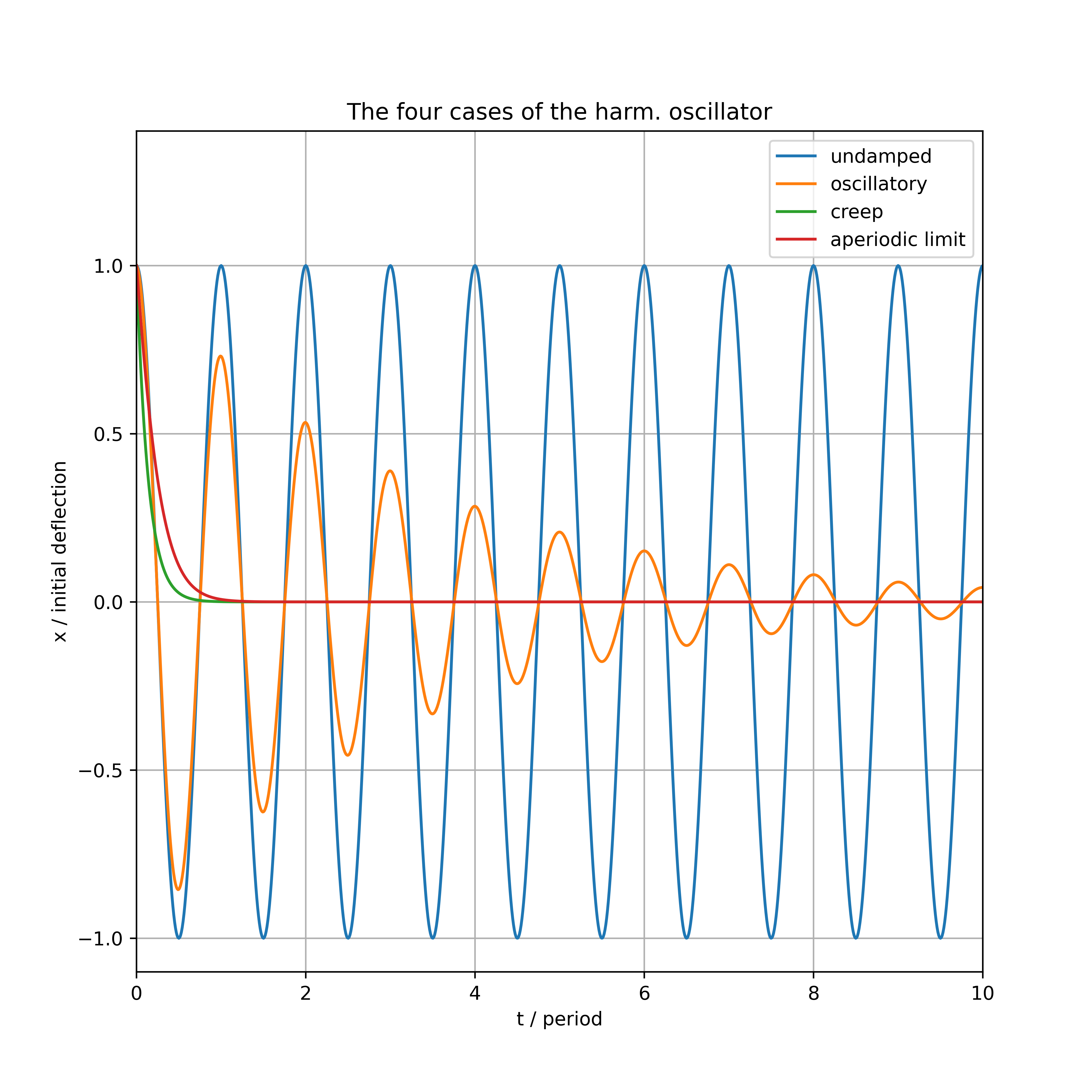
This case is called aperiodic limit. The four cases of the harmonic oscillator are shown in Fig. 2.1.
2.4.3 Powered case
Now you drive the system with the circular frequency $\omega$, modifying Eq. (2.91) too
\[ \begin{align} x'' + kx + 2dx' = y_0\exp\left(-i\omega t\right) \end{align} \]
with a real excitation amplitude $y_0 > 0$. If you use the approach $x = x_0e^{-i\omega t}$ again, you get
\[ \begin{align} -\omega^2x_0 + kx_0 - 2id\omega x_0 &= y_0\nonumber\\ \Leftrightarrow -\omega^2 + k - 2id\omega &= \frac{y_0}{x_0}\\ \Leftrightarrow \omega^2 - k + 2id\omega &= -\frac{y_0}{x_0}\\ \Leftrightarrow \omega^2 + 2id\omega + \left(\frac{y_0}{x_0} - k\right) &= 0.\tag{2.110}\label{eq_harm_osz_force_deriv_0} \end{align} \]
The amplitude is independent of time, therefore $\omega$ is real. For $x_0$ you now write down in polar coordinates
\[ \begin{align} x_0 = \left|x_0\right|\exp\left(i\phi\right), \end{align} \]
the real number $\phi$ is called the phase. If it is positive, the oscillator runs ahead of the excitation; if it is negative, the oscillator runs behind the excitation. Putting this into Eq. (2.110), you get
\[ \begin{align} \omega^2 + 2id\omega + \left(\frac{y_0}{\left|x_0\right|}e^{-i\phi} - k\right) &= \omega^2 + 2id\omega + \left(\frac{y_0}{\left|x_0\right|}\cos\left(\phi\right) - \frac{y_0}{\left|x_0\right|}i\sin\left(\phi\right) - k\right) = 0.\tag{2.112}\label{eq_harm_osz_force_deriv_1} \end{align} \]
$\omega$ is not an unknown here, it is given by the excitation. The unknowns are the reaction of the system $\left|x_0\right|, \phi$. To determine this, write down the real and imaginary parts of Equation. (2.112):
\[ \begin{align} \omega^2 + \left(\frac{y_0}{\left|x_0\right|}\cos\left(\phi\right) - k\right) &= 0,\tag{2.113}\label{eq_harm_osz_force_deriv_2}\\ 2d\omega - \frac{y_0}{\left|x_0\right|}\sin\left(\phi\right) &= 0 \Rightarrow 2d\omega = \frac{y_0}{\left|x_0\right|}\sin\left(\phi\right) \Rightarrow \left|x_0\right| = \frac{y_0}{2d\omega}\sin\left(\phi\right).\tag{2.114}\label{eq_harm_osz_force_deriv_3} \end{align} \]
If you put Eq. (2.114) in Eq. (2.113), you get
\[ \begin{align} \omega^2 + \left(\frac{y_0}{\frac{y_0}{2d\omega}\sin\left(\phi\right)}\cos\left(\phi\right) - k\right) &= 0\nonumber\\ \Leftrightarrow\omega^2 + \left(\frac{2d\omega}{\tan\left(\phi\right)} - k\right) &= 0\nonumber\\ \Leftrightarrow\omega^2\tan\left(\phi\right) + 2d\omega - k\tan\left(\phi\right) &= 0\nonumber\\ \Leftrightarrow\tan\left(\phi\right)\left(k - \omega^2\right) &= 2d\omega\nonumber\\ \Leftrightarrow\tan\left(\phi\right) &= \frac{2d\omega}{k - \omega^2}. \end{align} \]
The function
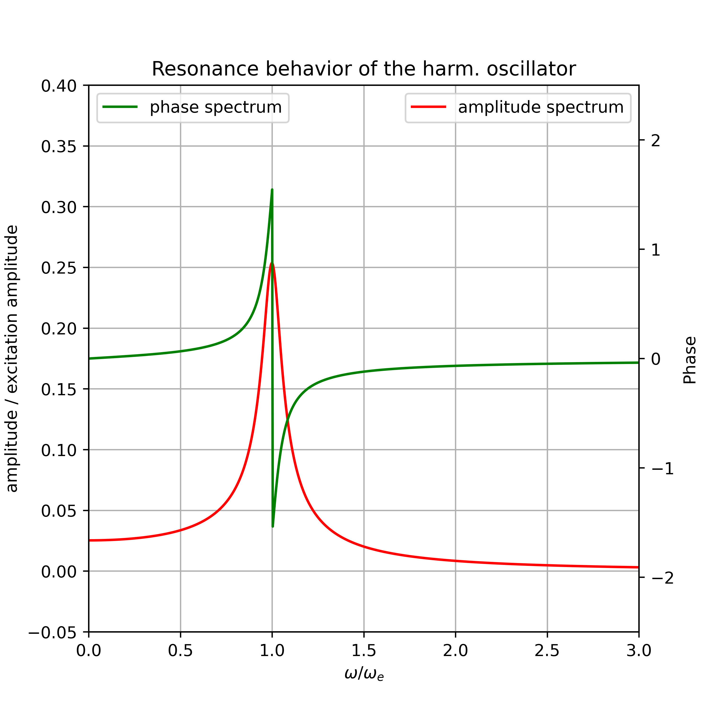
\[ \begin{align} \phi\left(\omega\right) = \arctan\left(\frac{2d\omega}{k - \omega^2}\right)\tag{2.116}\label{eq:harm_osz_phase} \end{align} \]
is called phase spectrum. Because $-\pi/2 < \phi < \pi/2$ holds
\[ \begin{align} \sin = \tan\cdot\cos = \tan\sqrt{1 - \sin^2} \Rightarrow \sin^2 = \tan^2 - \tan^2\sin^2 \Rightarrow \sin^2\left(1 + \tan^2\right) = \tan^2 \Rightarrow \sin = \frac{\tan}{\sqrt{1 + \tan^2}}. \end{align} \]
If you now set Eq. (2.116) in Eq. (2.114), you get
\[ \begin{align} \left|x_0\right| = \frac{y_0}{2d\omega}\sin\left(\phi\right) = \frac{y_0}{2d\omega}\frac{\tan\left(\phi\right)}{\sqrt{1 + \tan\left(\phi\right)^2}} = \frac{y_0}{2d\omega}\frac{\frac{2d\omega}{k - \omega^2}}{\sqrt{1 + \frac{4d^2\omega^2}{\left(k - \omega^2\right)^2}}} = \frac{y_0}{\left(k - \omega^2\right)\sqrt{1 + \frac{4d^2\omega^2}{\left(k - \omega^2\right)^2}}}. \end{align} \]
From this it follows
\[ \begin{align} \left|x_0\right| = \frac{y_0}{\sqrt{\left(k - \omega^2\right)^2 + 4d^2\omega^2}}. \end{align} \]
This function is called amplitude spectrum. One defines the auxiliary function $h$ by
\[ \begin{align} h\left(\omega\right) \coloneqq \left(k - \omega^2\right)^2 + 4d^2\omega^2 \Rightarrow h'\left(\omega\right) = -4\omega\left(k - \omega^2\right) + 8d^2\omega = -4\omega k + 4\omega^3 + 8d^2\omega. \end{align} \]
Setting the derivative to zero results in
\[ \begin{align} -4\omega k + 4\omega^3 + 8d^2\omega &\hastobe 0 \Rightarrow -4k + 4\omega^2 + 8d^2 = 0 \Rightarrow -k + \omega^2 + 2d^2 = 0\nonumber\\ \Rightarrow \omega^2 &= k - 2d^2. \end{align} \]
Here we limit ourselves to this case
\[ \begin{align} k - 2d^2 > 0 \Leftrightarrow d < \sqrt{\frac{k}{2}}. \end{align} \]
The frequency
\[ \begin{align} \omega_\text{res} \coloneqq \sqrt{k - 2d^2}\tag{2.123}\label{eq:resonancefrequency_damp} \end{align} \]
is called resonance frequency. For the second derivative of $h$ one obtains
\[ \begin{align} h''\left(\omega\right) = -4k + 12\omega^2 + 8d^2. \end{align} \]
From this it follows
\[ \begin{align} h''\left(\omega_\text{res}\right) = -4k + 12\left(k - 2d^2\right) + 8d^2 = -4k + 12k - 24d^2 + 8d^2 = 8k - 16d^2 = 8\left(k - 2d^2\right) > 0. \end{align} \]
$\omega_\text{res}$ ist also die Frequenz maximaler Amplitude. Man beachte den Unterschied zwischen Eigenfrequenz Glg. (2.97) und Resonanzfrequenz Glg. (2.123). Das Resonanzverhalten ist in Abb. 2.2 dargestellt.
The system considered so far in this section has exactly one degree of freedom, namely the generalized deflection $x$. Conceptually, however, many of the findings can be generalized to systems with many degrees of freedom. Such complex systems (houses, circuits, the climate) also have their own modes.