15 Vorticity and divergence

Let an arbitrary vector field $\mathbf{v}$ be given. The approach

\[ \begin{align} \mathbf{v} = \Delta\mathbf{w} \end{align} \]

with the boundary conditions

\[ \begin{align} \lim\limits_{\left|\mathbf{r}\right|\to\infty}\mathbf{w} = \mathbf{0} \end{align} \]

with a vector field $\mathbf{v}$ is clearly solvable for continuous $\mathbf{v}$, namely there are three independent Poisson equations

\[ \begin{align} v_i = \Delta w_i. \end{align} \]

According to Eq. (B.54) applies

\[ \begin{align} \Delta\mathbf{w} = \nabla\left(\nabla\cdot\mathbf{w}\right) - \nabla\times\left(\nabla\times\mathbf{w}\right). \end{align} \]

You define

\[ \begin{align} \chi \coloneqq\nabla\cdot\mathbf{w} \end{align} \]

as velocity potential, further one defines

\[ \begin{align} \mathbf{A} \coloneqq -\nabla\times\mathbf{w} \end{align} \]

as vector potential, then applies

\[ \begin{align} \mathbf{v} = \nabla\chi + \nabla\times\mathbf{A}. \end{align} \]

So you have a unique decomposition

\[ \begin{align} \mathbf{v} = \mathbf{v}_\text{nonrot} + \mathbf{v}_\text{nondiv}, & {} & \nabla\times\mathbf{v}_\text{nonrot} = \mathbf{0}, & {} & \nabla\cdot\mathbf{v}_\text{nondiv} = 0 \end{align} \]

made. The fact that this is always possible is the principal theorem of vector analysis. $\chi$ and $\mathbf{A}$ have a total of four components, but the wind field only has three. Therefore one can set another linear condition, here will

\[ \begin{align} \nabla\cdot\mathbf{A} = 0 \end{align} \]

chosen, it follows

\[ \begin{align} \nabla\times\mathbf{v} = \Delta\mathbf{A}. \end{align} \]

If you only look at the horizontal wind field

\[ \begin{align} \mathbf{v}_h \coloneqq\mathbf{v} - w\mathbf{k}, \end{align} \]

of course this also applies. Instead of the condition $\nabla\cdot\mathbf{A}\hastobe0$, one places the algebraic condition on the vector potential

\[ \begin{align} \mathbf{A}\hastobe\left(\mathbf{k}\cdot {\mathbf{A}}\right)\mathbf{k} \end{align} \]

and defines a current function $\psi = \psi\left(\varphi, \lambda\right) \coloneqq - \mathbf{k}\cdot \mathbf{A}$. Then applies

\[ \begin{align} \mathbf{v}_{h,{\text{nondiv}}} &= \nabla\times\left[-\mathbf{k}\psi\right]\stackrel{\href{ch-40-vector-analysis.html#eq:diff_op_rule_5}{\text{ Glg. (B.51)}}}{=} \mathbf{k}\times\nabla\psi.\tag{15.13}\label{eq:v_h_streamf} \end{align} \]

Expected to be checked

\[ \begin{align} \nabla\cdot\left(\mathbf{k}\times\nabla\psi\right)&\stackrel{\text{Glg. }\href{ch-40-vector-analysis.html#eq:diff_op_rule_9}{(B.55)}}{=} \nabla\psi\cdot\left(\nabla\times\mathbf{k}\right) - \mathbf{k}\cdot\left(\nabla\times\nabla\psi\right) = \mathbf{0}. \end{align} \]

You define

\[ \begin{align} \zetabi \coloneqq \nabla\times\mathbf{v}. \end{align} \]

It applies

\[ \begin{align} \zeta &\coloneqq \mathbf{k}\cdot\left(\nabla\times\mathbf{v}_h\right) = \mathbf{k}\cdot\left[\nabla\times\left(\mathbf{k}\times\nabla\psi\right)\right]\stackrel{\text{Glg. }\href{ch-40-vector-analysis.html#eq:diff_op_rule_7}{(B.53)}}{=}\Delta\psi. \end{align} \]

The divergence still applies

\[ \begin{align} \nabla\cdot\mathbf{v}_h = \Delta\chi. \end{align} \]

Note that $\zeta$ is not the magnitude of $\zetabi$, but the z-component of it.

15.1 Vorticity

The rotating base of the global coordinates is denoted by $\mathbf{e}_x, \mathbf{e}_y, \mathbf{e}_z$, so the velocity field is written as

\[ \begin{align} \mathbf{v} = u_x\mathbf{e}_x + u_y\mathbf{e}_y + u_z\mathbf{e}_z. \end{align} \]

You write

\[ \begin{align} \mathbf{U'} = \omegabi\times\mathbf{r} + \mathbf{v}, \end{align} \]

so $\mathbf{U'}$ is the field of particle velocities in coordinates at rest. It is composed of the proportion of the Earth's rotation $\omegabi\times\mathbf{r}$ and the wind field $\mathbf{v}$ measured relative to the rotating Earth. This follows

\[ \begin{align} \etabi \coloneqq\nabla\times\mathbf{v}' = \nabla\times\mathbf{v} + \nabla\times\left(\omegabi\times\mathbf{r}\right) = \zetabi + \mathbf{f}, \end{align} \]

it was

\[ \begin{align} \nabla\times\left(\omegabi\times\mathbf{r}\right)\stackrel{\href{ch-40-vector-analysis.html#eq:diff_op_rule_7}{\text{Glg. (B.53)}}}{=}\omegabi\left(\nabla\cdot\mathbf{r}\right) - \left(\omegabi\cdot\nabla\right)\mathbf{r} = 3\omegabi - \left(\omega\frac{\partial}{\partial z}\right)\mathbf{r} = 3\omegabi - \omegabi = 2\omegabi = \mathbf{f} \end{align} \]

used. The absolute vorticity $\eta$ is defined by the vertical component of the rotation of $\mathbf{v}'$. This is obtained as the dot product of $\nabla\times\mathbf{v}'$ with the vertical unit vector $\mathbf{k}$:

\[ \begin{align} \eta \coloneqq\mathbf{k}\cdot\left(\nabla\times\mathbf{v}\right) + \mathbf{k}\cdot\mathbf{f} = \zeta + f \end{align} \]

Recall that the Coriolis parameter is the vertical component of the Coriolis vector, not its magnitude. The portion of the absolute vorticity that is caused by the Earth's rotation is also referred to as planetary vorticity, while the portion that is caused by the wind field measured in rotating coordinates is referred to as relative vorticity.

The vorticity also has a clear meaning that is not initially as obvious as that of the divergence. Two examples are considered here.

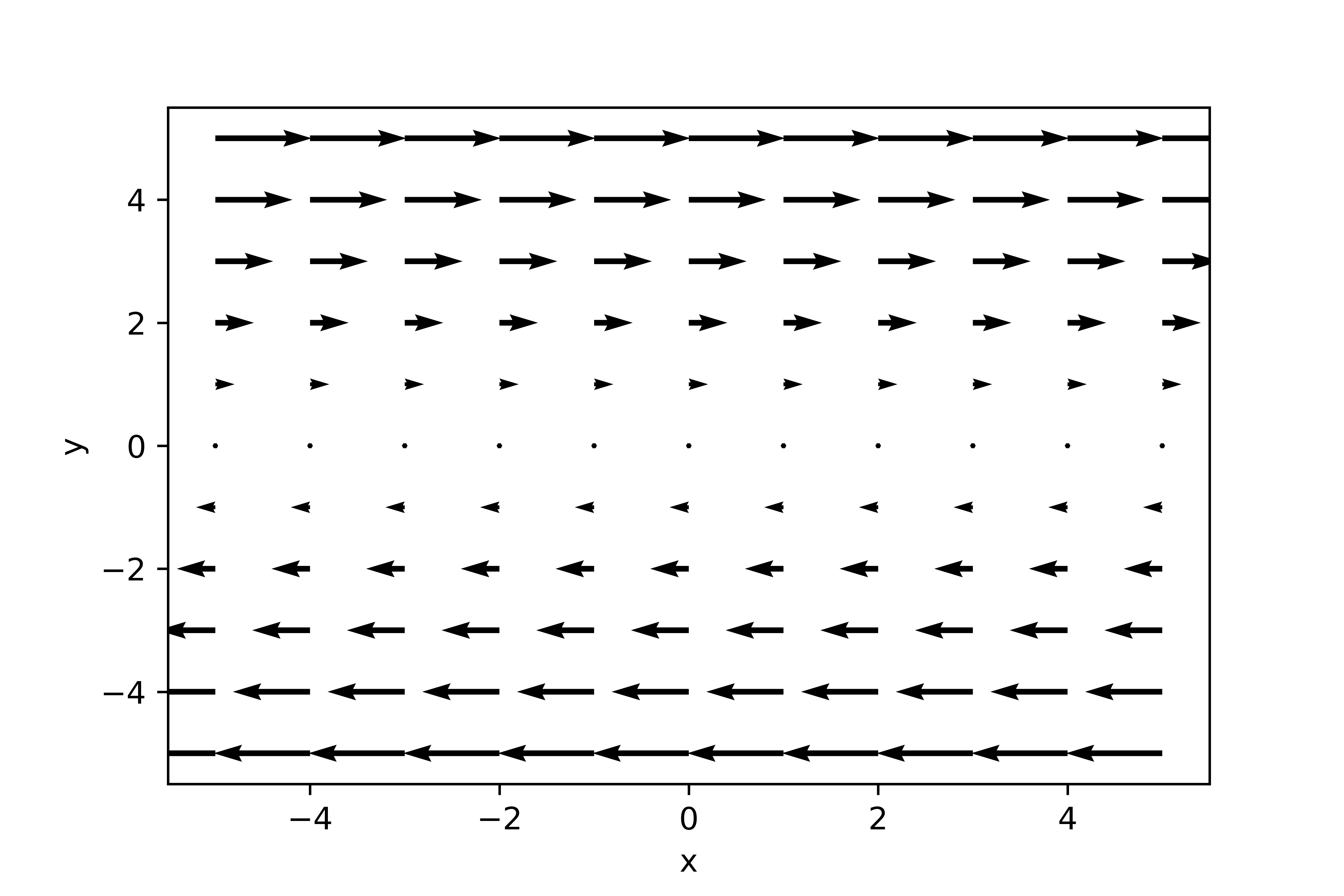
• Take the field $\mathbf{v} = \left(y, 0, 0\right)^T$. The streamlines of this field are not curved. Nevertheless, $\nabla\times\mathbf{v} = \left(0, 0, - 1\right)^T\not = \mathbf{0}$.
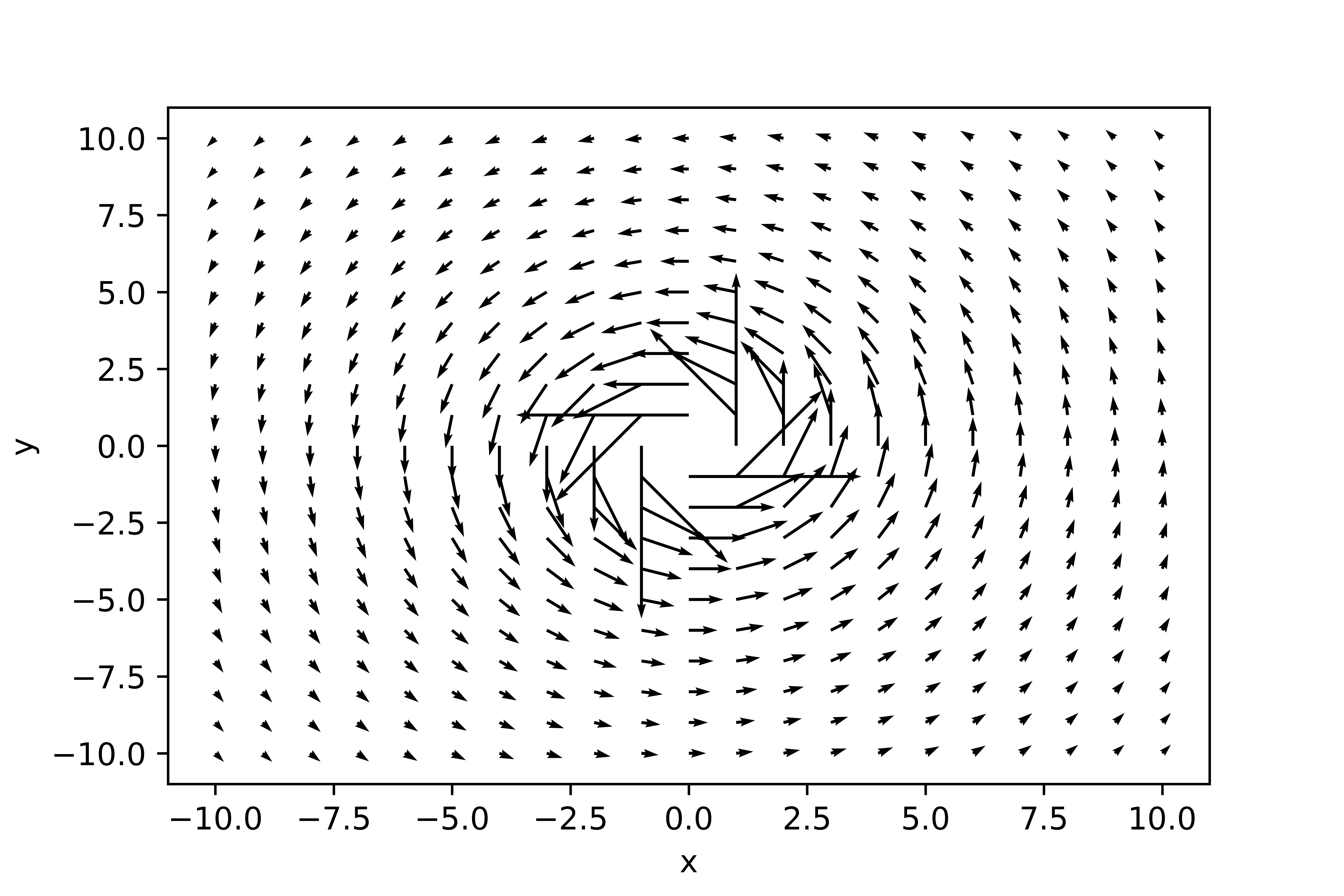
• Take the field $\mathbf{v} = \frac{1}{x^2 + y^2}\left(-y, x, 0\right)^T$. The field looks very much like a rotating field (see Fig. 15.1). Trotzdem gilt

  \[ \begin{align} \nabla\times\mathbf{v} &= \left(\frac{\partial}{\partial x}\frac{x}{x^2 + y^2} + \frac{\partial}{\partial y}\frac{y}{x^2 + y^2} \right)\mathbf{e}_z\nonumber\\ &= \left(\frac{1}{x^2 + y^2} - x2x\frac{1}{\left(x^2 + y^2\right)^2} + \frac{1}{x^2 + y^2} - y2y\frac{1}{\left(x^2 + y^2\right)^2}\right)\mathbf{e}_z = \mathbf{0}. \end{align} \]

To understand the true meaning of vorticity, it is best to imagine a 2D vector field $\mathbf{v}_h = \left(u, v\right)^T$ (in Cartesian coordinates). Take a rectangle $\left[-a, a\right]\times\left[-b, b\right]$. Let $\mathbf{s}$ be a curve that encloses this set in the positive mathematical sense of rotation. Then approximately with $\left(u, v\right)$ as the vector at the origin

\[ \begin{align} \int_{\mathbf{s}}^{}\mathbf{v}_h\cdot d\mathbf{s} &\approx 2a\left(u - b\frac{\partial u}{\partial y}\right) + 2b\left(v + a\frac{\partial v}{\partial x}\right) - 2a\left(u + b\frac{\partial u}{\partial y}\right) - 2b\left(v - a\frac{\partial v}{\partial x}\right)\nonumber\\ &= -2ba\frac{\partial u}{\partial y} + 2ba\frac{\partial v}{\partial x} - 2ab\frac{\partial u}{\partial y} + 2ba\frac{\partial v}{\partial x} = -4ba\frac{\partial u}{\partial y} + 4ab\frac{\partial v}{\partial x} = 4ab\left(\frac{\partial v}{\partial x} - \frac{\partial u}{\partial y}\right). \end{align} \]

The area of ​​the surface is $4ab$. If we consider the circulation of the vector field around a particle, then forms

\[ \begin{align} \lim\limits_{a, b\to 0}\frac{\int_{\mathbf{s}}^{}{\mathbf{v}_h\cdot d\mathbf{s}}}{4ab} = \frac{\partial v}{\partial x} - \frac{\partial u}{\partial y}, \end{align} \]

This results in the definition of the z component of the vortex strength. The components of the rotation therefore indicate how the flow flows around a small area in a plane perpendicular to the respective component. So there is a connection between circulation and vorticity. In integral form, this is the statement of Stokes Theorem:

\[ \begin{align} \int_{A}^{}\nabla\times\mathbf{v}\cdot d\mathbf{f} = \int_{\partial A}^{}\mathbf{v}\cdot d\mathbf{s}.\tag{15.26}\label{eq:satz_von_stokes} \end{align} \]

Just like the above consideration, Stokes' theorem links the vectorial curve integral along the edge of a surface with the vortex strength within the surface. A further illustration of vorticity is shown in the coming section.

15.1.1 Shear and curvature vorticity

Define o.b.d. A. in plane geometry, a right-handed orthonormal base $\mathbf{s}, \mathbf{n}, \mathbf{k}$, where $\mathbf{s}$ is parallel to the horizontal wind at the origin. This applies

\[ \begin{align} \mathbf{v} = \left(\begin{array}{c} V\cos\left(\beta\right)\\ V\sin\left(\beta\right)\\ w \end{array}\right)\tag{15.27}\label{eq:wind_natuerlich} \end{align} \]

with the horizontal wind speed $V$ and the vertical wind $w$. Here $\beta$ is the horizontal wind direction relative to $\mathbf{s}$. This follows for the vorticity

\[ \begin{align} \zeta &= \frac{\partial}{\partial s}V\sin\left(\beta\right) - \frac{\partial}{\partial n}V\cos\left(\beta\right) = \sin\left(\beta\right)\frac{\partial V}{\partial s} + V\frac{\partial\beta}{\partial s}\cos\left(\beta\right) - \cos\left(\beta\right)\frac{\partial V}{\partial n} + V\sin\left(\beta\right)\frac{\partial \beta}{\partial n}. \end{align} \]

At the coordinate origin $\beta = 0$, so there you have

\[ \begin{align} \zeta = V\frac{\partial\beta}{\partial s} - \frac{\partial V}{\partial n}. \end{align} \]

The first term $V\frac{\partial\beta}{\partial s}$ is called curvature vorticity. It is greater than zero if the streamline is curved to the left, equal to zero if the streamline is straight, and less than zero if the streamline is curved to the right. The term $-\frac{\partial V}{\partial n}$ is called shear vorticity. It is greater than zero if the wind speed increases to the right of the wind direction. In particular, one sees that a flow field with curved streamlines can be rotation-free and one with straight streamlines can be rotation-affected.

15.1.2 circulation rate

Let $A$ be an arbitrarily shaped surface in space, then the circulation $S$ of the wind field $\mathbf{v}$ around $A$ at time $t$ is defined by

\[ \begin{align} S\left(t\right) \coloneqq \int_{\partial A}\mathbf{v}\cdot d\mathbf{s} = \int_0^1\mathbf{v}\left(\mathbf{r}\left(\tau\right), t\right)\cdot\frac{d\mathbf{r}}{d\tau}d\tau, \end{align} \]

where $\mathbf{r}\left(\tau\right)$ is a function defined on the interval $\left[0, 1\right]$ that traverses the boundary of $A$. If the surface $A$ moves with the wind field, the circulation $S$ also changes by $A$, i.e

\[ \begin{align} \md{S} = \md{}\int_0^1\mathbf{v}\left(\mathbf{r}\left(\tau\right), t\right)\cdot\frac{d\mathbf{r}}{d\tau}d\tau = \int_0^1\md{\mathbf{v}}\cdot\frac{d\mathbf{r}}{d\tau}d\tau + \int_0^1\mathbf{v}\cdot\md{}\left(\frac{d\mathbf{r}}{d\tau}\right)d\tau. \end{align} \]

In order to determine the second integral in more detail, one prepares

\[ \begin{align} \frac{d\mathbf{r}}{d\tau} &= \lim_{\Delta \to 0}\frac{\mathbf{r}\left(\tau + \Delta\right) - \mathbf{r}\left(\tau\right)}{\Delta}\nonumber\\ \Rightarrow \md{}\frac{d\mathbf{r}}{d\tau} &= \lim_{\Delta \to 0}\frac{\md{\mathbf{r}}\left(\tau + \Delta\right) - \md{\mathbf{r}}\left(\tau\right)}{\Delta} = \lim_{\Delta \to 0}\frac{\mathbf{v}\left(\mathbf{r}\left(\tau + \Delta\right)\right) - \mathbf{v}\left(\mathbf{r}\left(\tau\right)\right)}{\Delta}\nonumber\\ &= \left(\frac{d\mathbf{r}}{d\tau}\cdot\nabla\right)\mathbf{v} \end{align} \]

firmly. Define $\mathbf{v}\left(\tau\right) \coloneqq \mathbf{v}\left(\mathbf{r}\left(\tau\right), t\right)$, then holds

\[ \begin{align} \left(\frac{d\mathbf{r}}{d\tau}\cdot\nabla\right)\mathbf{v} = \frac{d\mathbf{v}}{d\tau}, \end{align} \]

with what you

\[ \begin{align} \int_0^1\mathbf{v}\cdot\md{}\left(\frac{d\mathbf{r}}{d\tau}\right)d\tau = \int_0^1\mathbf{v}\cdot\frac{d\mathbf{v}}{d\tau}d\tau = \frac{1}{2}\left[\mathbf{v}^2\right]_0^1 = 0 \end{align} \]

because due to the closedness of the curve $\mathbf{v}\left(0\right) = \mathbf{v}\left(1\right)$. Using Stokes' theorem follows

\[ \begin{align} \md{S} = \int_A\nabla\times\mathbf{F}\cdot d\mathbf{n}, \end{align} \]

where $\mathbf{F}$ is the sum of all acting forces. So conservative forces do not change the circulation. With

\[ \begin{align} \nabla\times\left(-\frac{1}{\rho}\nabla p\right) & \stackrel{\href{ch-40-vector-analysis.html#eq:diff_op_rule_5}{\text{Glg. (B.51)}}}{=} \frac{1}{\rho^2}\nabla\rho\times\nabla p,\\ \nabla\times\mathbf{v}\times\mathbf{f} & \stackrel{\href{ch-40-vector-analysis.html#eq:diff_op_rule_7}{\text{Glg. (B.53)}}}{=} \left(\mathbf{f}\cdot\nabla\right)\mathbf{v} - \mathbf{f}\nabla\cdot\mathbf{v} \end{align} \]

follows

In IS this applies in barotropic ideal media

\[ \begin{align} \md{S} = 0 \Leftrightarrow S = \text{const.}\tag{15.39}\label{eq:circ_theorem_mod_1} \end{align} \]

15.1.3 Vorticity equation

The momentum equation Eq. (8.101) is

\[ \begin{align} \frac{\partial\mathbf{v}}{\partial t} &= -\frac{1}{\rho}\nabla p + \mathbf{v}\times\etabi - \nabla k + \mathbf{g} + \mathbf{f}_R. \end{align} \]

Now you apply the operator $\nabla\times $ to the individual terms:

\[ \begin{align} \nabla\times\frac{\partial\mathbf{v}}{\partial t} &\stackrel{\href{ch-40-vector-analysis.html#eq:diff_op_rule_4}{\text{Glg. (B.50)}}}{=} \frac{\partial}{\partial t}\left(\nabla\times\mathbf{v}\right)\\ \nabla\times\left(-\frac{1}{\rho}\nabla p\right) &= -\nabla\times\left(\frac{1}{\rho}\nabla p\right) \stackrel{\href{ch-40-vector-analysis.html#eq:diff_op_rule_5}{\text{Glg. (B.51)}}}{=} -\frac{1}{\rho^2}\nabla p\times\nabla\rho\\ \nabla\times\left(\mathbf{v}\times\etabi\right) &\stackrel{\href{ch-40-vector-analysis.html#eq:diff_op_rule_7}{\text{Glg. (B.53)}}}{=} -\left(\mathbf{v}\cdot\nabla\right)\etabi - \etabi\nabla\cdot\mathbf{v} + \left(\etabi\cdot\nabla\right)\mathbf{v}\\ \nabla\times\nabla k &\stackrel{\href{ch-40-vector-analysis.html#eq:diff_op_rule_1}{\text{Glg. (B.47)}}}{=} \mathbf{0}\\ \nabla\times\mathbf{g} &= \nabla\times\left(-\nabla\Phi\right) \stackrel{\href{ch-40-vector-analysis.html#eq:diff_op_rule_1}{\text{Glg. (B.47)}}}{=} \mathbf{0} \end{align} \]

Therefore applies

\[ \begin{align} \frac{\partial}{\partial t}\left(\nabla\times\mathbf{v}\right) &= \frac{1}{\rho^2}\nabla\rho\times\nabla p - \left(\mathbf{v}\cdot\nabla\right)\etabi - \etabi\nabla\cdot\mathbf{v} + \left(\etabi\cdot\nabla\right)\mathbf{v} + \nabla\times\mathbf{f}_R.\tag{15.46}\label{eq:vorticity_eq_3d} \end{align} \]

15.1.3.1 Formulation in geographical coordinates

By projecting onto the local perpendicular one obtains

\[ \begin{align} \frac{\partial\zeta}{\partial t} &= \mathbf{k}\cdot\left[\frac{1}{\rho^2}\nabla\rho\times\nabla p - \left(\mathbf{v}\cdot\nabla\right)\etabi - \etabi\nabla\cdot\mathbf{v} + \left(\etabi\cdot\nabla\right)\mathbf{v} + \nabla\times\mathbf{f}_R\right]\nonumber\\ \Leftrightarrow\frac{\partial\zeta}{\partial t} &= \mathbf{k}\cdot\left[\frac{1}{\rho^2}\nabla\rho\times\nabla p - \etabi\nabla\cdot\mathbf{v} - \left(\mathbf{v}\cdot\nabla\right)\etabi + \left(\etabi\cdot\nabla\right)\mathbf{v} + \nabla\times\mathbf{f}_R\right]\nonumber\\ \Leftrightarrow\frac{\partial\zeta}{\partial t} &= \mathbf{k}\cdot\left[\frac{1}{\rho^2}\nabla\rho\times\nabla p - \etabi\nabla\cdot\mathbf{v} + \left(\etabi\cdot\nabla\right)\mathbf{v} - \left(\mathbf{v}\cdot\nabla\right)\etabi + \nabla\times\mathbf{f}_R\right]\nonumber\\ \Rightarrow\frac{\partial\zeta}{\partial t} &= \frac{1}{\rho^2}\mathbf{k}\cdot\left(\nabla\rho\times\nabla p\right) - \eta\nabla\cdot\mathbf{v} + \mathbf{k}\cdot\left[\left(\etabi\cdot\nabla\right)\mathbf{v}\right] - \mathbf{k}\cdot\left[\left(\mathbf{v}\cdot\nabla\right)\etabi\right] + \mathbf{k}\cdot\nabla\times\mathbf{f}_R. \end{align} \]

One first calculates with Eq. (B.58)

\[ \begin{align} \left(\etabi\cdot\nabla\right)w = \left(\etabi\cdot\nabla\right)\left(\mathbf{v}\cdot\mathbf{k}\right) &= \mathbf{k}\cdot\left[\left(\etabi\cdot\nabla\right)\mathbf{v}\right] + \mathbf{v}\cdot\left[\left(\etabi\cdot\nabla\right)\mathbf{k}\right]\nonumber\\ \Rightarrow\mathbf{k}\cdot\left[\left(\etabi\cdot\nabla\right)\mathbf{v}\right] &= \left(\etabi\cdot\nabla\right)w - \mathbf{v}\cdot\left[\left(\etabi\cdot\nabla\right)\mathbf{k}\right],\\ \mathbf{v}\cdot\nabla\eta = \left(\mathbf{v}\cdot\nabla\right)\left(\etabi\cdot\mathbf{k}\right) &= \etabi\cdot\left[\left(\mathbf{v}\cdot\nabla\right)\mathbf{k}\right] + \mathbf{k}\cdot\left[\left(\mathbf{v}\cdot\nabla\right)\etabi\right]\nonumber\\ \Rightarrow\mathbf{k}\cdot\left[\left(\mathbf{v}\cdot\nabla\right)\etabi\right] &= \mathbf{v}\cdot\nabla\eta - \etabi\cdot\left[\left(\mathbf{v}\cdot\nabla\right)\mathbf{k}\right]. \end{align} \]

Therefore applies

\[ \begin{align} \frac{\partial\zeta}{\partial t} &= \frac{1}{\rho ^2}\mathbf{k}\cdot\left(\nabla\rho\times\nabla p\right) - \eta\nabla\cdot\mathbf{v} + \left(\etabi\cdot\nabla\right)w - \mathbf{v}\cdot\left[\left(\etabi\cdot\nabla\right)\mathbf{k}\right] - \mathbf{v}\cdot\nabla\eta + \etabi\cdot\left[\left(\mathbf{v}\cdot\nabla\right)\mathbf{k}\right] + \mathbf{k}\cdot\nabla\times\mathbf{f}_R. \end{align} \]

The findings in Section B.2.1 apply

\[ \begin{align} \frac{\partial\mathbf{k}}{\partial x} = \frac{\mathbf{i}}{r}, & {} & \frac{\partial\mathbf{k}}{\partial y} = \frac{\mathbf{j}}{r}, & {} & \frac{\partial\mathbf{k}}{\partial z} = \mathbf{0}. \end{align} \]

Thus follows

\[ \begin{align} \frac{\partial\zeta}{\partial t} &= \frac{1}{\rho ^2}\mathbf{k}\cdot\left(\nabla\rho\times\nabla p\right) - \eta\nabla\cdot\mathbf{v} + \etabi\cdot\nabla w - \mathbf{v}\cdot\left(\eta_x\frac{\partial\mathbf{k}}{\partial x} + \eta_y\frac{\partial\mathbf{k}}{\partial y}\right) - \mathbf{v}\cdot\nabla\eta + \etabi\cdot\left(u\frac{\partial\mathbf{k}}{\partial x} + v\frac{\partial\mathbf{k}}{\partial y}\right) + \mathbf{k}\cdot\nabla\times\mathbf{f}_R\nonumber\\ \Leftrightarrow\frac{\partial\zeta}{\partial t} &= \frac{1}{\rho ^2}\mathbf{k}\cdot\left(\nabla\rho\times\nabla p\right) - \eta\nabla\cdot\mathbf{v} + \etabi\cdot\nabla w \textcolor{blue}{- \frac{u\eta_x}{r}} \textcolor{red}{- \frac{v\eta_y}{r}} - \mathbf{v}\cdot\nabla\eta \textcolor{blue}{+ \frac{\eta_xu}{r}} \textcolor{red}{+ \frac{\eta_yv}{r}} + \mathbf{k}\cdot\nabla\times\mathbf{f}_R. \end{align} \]

The terms marked in color cancel each other out. Therefore applies

\[ \begin{align} \frac{\partial\zeta}{\partial t} &= \frac{1}{\rho ^2}\mathbf{k}\cdot\left(\nabla\rho\times\nabla p\right) - \eta\nabla\cdot\mathbf{v} + \etabi\cdot\nabla w - \mathbf{v}\cdot\nabla\eta + \mathbf{k}\cdot\nabla\times\mathbf{f}_R. \end{align} \]

The vorticity equation is finally:

15.1.3.2 Interpretation of the terms

If you neglect the friction, you get

\[ \begin{align} \frac{\partial\zeta}{\partial t} = -\mathbf{v}\cdot\nabla\eta - \eta\nabla\cdot\mathbf{v} + \etabi\cdot\nabla w + \frac{1}{\rho ^2}\mathbf{k}\cdot\left(\nabla\rho\times\nabla p\right). \end{align} \]

If one assumes a flat geofluid and introduces a horizontal wind vector $\mathbf{v}_h$, it follows

\[ \begin{align} \frac{\partial\zeta}{\partial t} &= -\mathbf{v}\cdot\nabla\eta - \eta\nabla\cdot\mathbf{v}_h - \eta\frac{\partial w}{\partial z} + \etabi_h\cdot\nabla_hw + \eta\frac{\partial w}{\partial z} + \frac{1}{\rho ^2}\mathbf{k}\cdot\left(\nabla\rho\times\nabla p\right)\nonumber\\ &= \underbrace{-\mathbf{v}\cdot\nabla\eta - \eta\nabla\cdot\mathbf{v}_h + \etabi_h\cdot\nabla_hw}_\text{Advektion} + \underbrace{\frac{1}{\rho^2}\mathbf{k}\cdot\left(\nabla\rho\times\nabla p\right)}_\text{Solenoidterm}. \end{align} \]

The so-called solenoid term arises from the rotation of the pressure gradient acceleration. The rotation of $\nabla p$ is zero. A closed line integral over $-\nabla p\cdot d\mathbf{n}$ therefore disappears. However, due to the location dependence of the density, $\int_{\partial\Omega\subseteq\mathbb{R}^2}-\frac{1}{\rho}\nabla p\cdot d\mathbf{n} \not= 0$ can apply. A particle that moves on a closed path, for example a circular path, can be accelerated or decelerated by the pressure gradient, which changes the vorticity.

So apart from the solenoid term, vorticity is only generated by momentum advection. This can be broken down as follows:

\[ \begin{align} \frac{\partial\zeta}{\partial t}_\text{adv} &= \underbrace{-\mathbf{v}\cdot\nabla\eta}_\text{Vorticityadvektion} \underbrace{- \eta\nabla\cdot\mathbf{v}_h}_\text{Divergenzterm} \underbrace{+ \etabi_h\cdot\nabla_hw}_\text{Drehterm} \end{align} \]

The Rotation term describes the generation of vertical vorticity by horizontal vorticity and a horizontal gradient of the vertical velocity. It applies

\[ \begin{align} \etabi_h\cdot\nabla_hw = \zeta_x\frac{\partial w}{\partial x} + \zeta_y\frac{\partial w}{\partial y}. \end{align} \]

O.B.d. A. the y-axis of the KS is aligned with $\zetabi_h$, resulting in

\[ \begin{align} \etabi_h\cdot\nabla_hw = \zeta_y\frac{\partial w}{\partial y} \end{align} \]

leads. Now assume a convective tube with amplitude $W$ and variance $\sigma^2$, i.e

\[ \begin{align} w = w\left(x, y\right) = W\exp\left(-\frac{x^2 + y^2}{2\sigma^2}\right). \end{align} \]

The KS was again placed in the center of the tube. From this it follows

\[ \begin{align} \frac{\partial w}{\partial y} = -\frac{Wy}{\sigma^2}\exp\left(-\frac{x^2 + y^2}{2\sigma^2}\right). \end{align} \]

For the y-component of the relative vorticity applies

\[ \begin{align} \zeta_y = \frac{\partial u}{\partial z} - \frac{\partial w}{\partial x}. \end{align} \]

From this it follows

\[ \begin{align} \etabi_h\cdot\nabla_hw &= \left(\frac{\partial u}{\partial z} - \frac{\partial w}{\partial x}\right)\frac{\partial w}{\partial y} = -\frac{Wy}{\sigma^2}\left[\frac{\partial u}{\partial z} + \frac{Wx}{\sigma^2}\exp\left(-\frac{x^2 + y^2}{2\sigma^2}\right)\right]\exp\left(-\frac{x^2 + y^2}{2\sigma^2}\right). \end{align} \]

If you insert $x = 0$, $y = \pm\sigma$ and approximate all exponential terms by 1/2, it follows

\[ \begin{align} \etabi_h\cdot\nabla_hw &= \mp\frac{W}{2\sigma}\frac{\partial u}{\partial z}. \end{align} \]

Most of the time $\frac{\partial u}{\partial z} > 0$. Thus, the rotation term produces cyclonic vorticity south of the convective tube and anticyclonic vorticity north of the tube. The scale analysis obtained for the case of very strong convection is $\sigma \sim 50$ m, $W \sim 10 $m/s and $\frac{\partial u}{\partial z} \sim \frac{20\text{ m/s}}{2\text{ km}} = 1\cdot 10^{-2}$ 1/s

\[ \begin{align} \etabi_h\cdot\nabla_hw \sim \frac{10}{100}10^{-2}\text{ 1/s}^2 = 10^{-3}\text{ 1/s}^2. \end{align} \]

This is seven orders of magnitude stronger than the synoptic-scale vorticity tendency. This mechanism is important for the formation of tornadoes. The rotation term is all the more effective,

• the stronger the vertical shear of the horizontal wind is, and
• the stronger the convection.

15.1.3.3 Barotropic vorticity equation

In the barotropic case, the solenoid term is omitted and the vertical shear of the horizontal wind is ignored (see section 13.8).

This is the so-called barotropic vorticity equation. In the case of incompressibility, especially in the case of SWEs, $\nabla\cdot\mathbf{v} = 0$, from which it follows

\[ \begin{align} \frac{\partial\zeta}{\partial t} = -\mathbf{v}_h\cdot\nabla\eta + \etabi\cdot\nabla w\Rightarrow\frac{d\eta}{dt} = \etabi\cdot\nabla w. \end{align} \]

Neglecting the horizontal gradients of $w$, it follows

\[ \begin{align} \md{\eta} = \eta\frac{\partial w}{\partial z}.\tag{15.68}\label{eq:vorticit_z_baro_swes_pre} \end{align} \]

You bet

\[ \begin{align} \nabla\cdot\mathbf{v} &= \nabla\cdot\mathbf{v}_h + \frac{\partial w}{\partial z} = 0 \end{align} \]

one, where a width-independent curvature term $\propto\frac{w}{r}$ was neglected, follows

In the incompressible, horizontally divergence-free, barotropic case (in addition, the vertical shear of the horizontal wind was ignored), the absolute vorticity is a conserved quantity.

15.1.3.4 Vorticity equation in the p-system

Now the same thing should be done in the p-system. The momentum equations (13.132) - (13.133) in the p-system are vectorial

\[ \begin{align} \frac{\partial\mathbf{v}_h}{\partial t} &= -\nabla\phi - \frac{1}{2}\nabla\left(\mathbf{v}_h\cdot\mathbf{v}_h\right) + \mathbf{v}_h\times\etabi' - \omega\frac{\partial\mathbf{v}_h}{\partial p} + \nabla\times\mathbf{f}_R^{(H)}. \end{align} \]

The modified absolute vorticity $\etabi'$ was given by

\[ \begin{align} \etabi' \coloneqq f\mathbf{k} + \nabla\times\mathbf{v}_h \end{align} \]

defined. Now you apply the operator $\nabla\times $ to the individual terms:

\[ \begin{align} \nabla\times\frac{\partial\mathbf{v}_h}{\partial t}&\stackrel{\href{ch-40-vector-analysis.html#eq:diff_op_rule_4}{\text{Glg. (B.50)}}}{=} \frac{\partial}{\partial t}\nabla\times\mathbf{v}_h\\ \nabla\times\nabla\phi&\stackrel{\href{ch-40-vector-analysis.html#eq:diff_op_rule_1}{\text{Glg. (B.47)}}}{=} \mathbf{0}\\ \nabla\times\mathbf{g}&\stackrel{\href{ch-40-vector-analysis.html#eq:diff_op_rule_1}{\text{Glg. (B.47)}}}{=} \mathbf{0}\\ \nabla\times\nabla\left(\mathbf{v}_h\cdot\mathbf{v}_h\right)&\stackrel{\href{ch-40-vector-analysis.html#eq:diff_op_rule_1}{\text{Glg. (B.47)}}}{=} \mathbf{0}\\ \nabla\times\left(\mathbf{v}_h\times\etabi'\right)&\stackrel{\href{ch-40-vector-analysis.html#eq:diff_op_rule_7}{\text{Glg. (B.53)}}}{=} -\left(\mathbf{v}_h\cdot\nabla\right)\etabi' - \etabi'\nabla\cdot\mathbf{v}_h + \left(\etabi'\cdot\nabla\right)\mathbf{v}_h\\ \nabla\times\left(\omega\frac{\partial\mathbf{v}_h}{\partial p}\right)&\stackrel{\href{ch-40-vector-analysis.html#eq:diff_op_rule_5}{\text{Glg. (B.51)}}}{=} \omega\nabla\times\frac{\partial\mathbf{v}_h}{\partial p} - \frac{\partial\mathbf{v}_h}{\partial p}\times\nabla\omega \end{align} \]

Therefore applies

\[ \begin{align} \frac{\partial}{\partial t}\nabla\times\mathbf{v}_h &= -\left(\mathbf{v}_h\cdot\nabla\right)\etabi' - \etabi'\nabla\cdot\mathbf{v}_h + \left(\etabi'\cdot\nabla\right)\mathbf{v}_h + \omega\nabla\times\frac{\partial\mathbf{v}_h}{\partial p} - \frac{\partial\mathbf{v}_h}{\partial p}\times\nabla\omega + \nabla\times\mathbf{f}_R^{(H)}. \end{align} \]

15.1.3.5 Formulation in geographical coordinates

By projecting onto the local perpendicular $\mathbf{k}$ one obtains

\[ \begin{align} \frac{\partial\zeta}{\partial t} &= -\mathbf{k}\cdot\left[\left(\mathbf{v}_h\cdot\nabla\right)\etabi'\right] - \left(f + \zeta\right)\nabla\cdot\mathbf{v}_h + \mathbf{k}\cdot\left[\left(\etabi'\cdot\nabla\right)\mathbf{v}_h\right]\nonumber\\ & - \omega\frac{\partial\zeta}{\partial p} + \mathbf{k}\cdot\left[\frac{\partial\mathbf{v}_h}{\partial p}\times\nabla\omega\right] + \mathbf{k}\cdot\nabla\times\mathbf{f}_R^{(H)}. \end{align} \]

One first calculates with Eq. (B.58)

\[ \begin{align} 0 = \left(\etabi'\cdot\nabla\right)\left(\mathbf{v}_h\cdot\mathbf{k}\right) &= \mathbf{k}\cdot\left[\left(\etabi'\cdot\nabla\right)\mathbf{v}_h\right] + \mathbf{v}_h\cdot\left[\left(\etabi'\cdot\nabla\right)\mathbf{k}\right]\nonumber\\ \Rightarrow\mathbf{k}\cdot\left[\left(\etabi'\cdot\nabla\right)\mathbf{v}_h\right] &= -\mathbf{v}_h\cdot\left[\left(\etabi'\cdot\nabla\right)\mathbf{k}\right],\\ \mathbf{v}_h\cdot\nabla\eta = \left(\mathbf{v}_h\cdot\nabla\right)\left(\etabi'\cdot\mathbf{k}\right) &= \etabi'\cdot\left[\left(\mathbf{v}_h\cdot\nabla\right)\mathbf{k}\right] + \mathbf{k}\cdot\left[\left(\mathbf{v}_h\cdot\nabla\right)\etabi'\right]\nonumber\\ \Rightarrow\mathbf{k}\cdot\left[\left(\mathbf{v}_h\cdot\nabla\right)\etabi'\right] &= \mathbf{v}_h\cdot\nabla\eta - \etabi'\cdot\left[\left(\mathbf{v}_h\cdot\nabla\right)\mathbf{k}\right]. \end{align} \]

The findings in Section B.2.1 apply

\[ \begin{align} \frac{\partial\mathbf{k}}{\partial x} = \frac{\mathbf{i}}{r}, & {} & \frac{\partial\mathbf{k}}{\partial y} = \frac{\mathbf{j}}{r}, & {} & \frac{\partial\mathbf{k}}{\partial z} = \mathbf{0}. \end{align} \]

Thus follows

\[ \begin{align} \mathbf{v}_h\cdot\left[\left(\etabi'\cdot\nabla\right)\mathbf{k}\right] &= \etabi'\cdot\left[\left(\mathbf{v}_h\cdot\nabla\right)\mathbf{k}\right]. \end{align} \]

The vorticity equation in the p-system is:

If you calculate the vorticity of the geostrophic wind field you get

\[ \begin{align} \zeta_g = \frac{1}{f}\frac{\partial^2\phi}{\partial x^2} + \frac{1}{f}\frac{\partial^2\phi}{\partial y^2} - \frac{\beta}{f^2}\frac{\partial\phi}{\partial y} + \frac{\tan\left(\varphi\right)u}{r} = \frac{1}{f}\Delta_h\phi + \frac{\beta}{f}u + \frac{\tan\left(\varphi\right)u}{r}.\tag{15.86}\label{eq:geostro_vort_skal} \end{align} \]

For the first term applies

\[ \begin{align} \mathcal{O}\left(\frac{1}{f}\Delta\phi\right) = \mathcal{O}\left(\frac{1}{f}\frac{\Delta p}{\rho L^2}\right) = 10^{-5}\:\frac{1}{\text{s}}. \end{align} \]

The term of the $\beta $effect has a magnitude of $10^{-6}$ 1/s in mid-latitudes. Therefore, a common approximation in the extratropics is to approximate the vorticity by the geostrophic vorticity and to neglect the term of the beta effect.

15.1.3.6 Barotropic vorticity equation in the p-system

If you delete from Eq. (15.85) the friction and all terms containing vertical gradients are obtained

\[ \begin{align} \frac{\partial\zeta}{\partial t} &= -v\beta - \left(f + \zeta\right)\nabla\cdot\mathbf{v}_h - \mathbf{v}_h\cdot\nabla\zeta. \end{align} \]

In the barotropic medium, $\partial w/\partial z \sim \partial\omega/\partial p$ is now constant in height. Under kinematic boundary conditions

\[ \begin{align} \omega\left(p = 0\right) = \omega\left(p_\text{surface}\right) = 0 \end{align} \]

thus follows

\[ \begin{align} \frac{\partial\omega}{\partial p} = \frac{\omega\left(p_\text{surface}\right) - \omega\left(p = 0\right)}{p_\text{surface}} = 0. \end{align} \]

Due to Eq. (13.129) now also applies

\[ \begin{align} \nabla\cdot\mathbf{v}_h = -\frac{\partial\omega}{\partial p} = 0.\tag{15.91}\label{eq:div_free_baro_vort} \end{align} \]

From this you get the barotropic vorticity equation in the p-system

Other forms of this equation are:

\[ \begin{align} \frac{\partial\eta}{\partial t} &= -v\beta - \mathbf{v}_h\cdot\nabla\zeta,\\ \frac{D_h\zeta}{Dt} &= -v\beta,\\ \frac{D_h\eta}{Dt} &= 0. \end{align} \]

Due to Eq. (15.91) $\mathbf{v}_h$ can be represented by a stream function $\psi = \psi\left(\phi, \lambda\right)$, i.e

\[ \begin{align} \mathbf{v}_h &\stackrel{\href{#eq:v_h_streamf}{\text{Glg. (15.13)}}}{=} \mathbf{k}\times\nabla\psi = -\frac{\partial\psi}{\partial y}\mathbf{i} + \frac{\partial\psi}{\partial x}\mathbf{j} = -\frac{\partial\psi}{a\partial\phi}\mathbf{i} + \frac{\partial\psi}{a\cos\left(\phi\right)\partial\lambda}\mathbf{j}\nonumber\\ \Rightarrow u &= -\frac{\partial\psi}{a\partial\phi},\\ v &= \frac{\partial\psi}{a\cos\left(\phi\right)\partial\lambda}. \end{align} \]

From this it follows

\[ \begin{align} \zeta = \Delta\psi. \end{align} \]

Putting this into Eq. (15.92), you get

\[ \begin{align} \frac{\partial\zeta}{\partial t} &= -v\beta - u\frac{\partial\zeta}{a\cos\left(\phi\right)\partial\lambda} - v\frac{\partial\zeta}{a\partial\phi}\nonumber\\ \Leftrightarrow\Delta\frac{\partial\psi}{\partial t} &= -\frac{\partial\psi}{a\cos\left(\phi\right)\partial\lambda}\beta + \frac{\partial\psi}{a\partial\phi}\frac{\partial\zeta}{a\cos\left(\phi\right)\partial\lambda} - \frac{\partial\psi}{a\cos\left(\phi\right)\partial\lambda}\frac{\partial\zeta}{a\partial\phi}\nonumber\\ \Leftrightarrow\Delta\frac{\partial\psi}{\partial t} &= -\frac{\partial\psi}{a\cos\left(\phi\right)\partial\lambda}\beta + \frac{1}{a^2\cos\left(\phi\right)}\left(\frac{\partial\psi}{\partial\phi}\frac{\partial\zeta}{\partial\lambda} - \frac{\partial\psi}{\partial\lambda}\frac{\partial\zeta}{\partial\phi}\right)\nonumber\\ \Leftrightarrow\Delta\frac{\partial\psi}{\partial t} &= -\frac{\partial\psi}{a\cos\left(\phi\right)\partial\lambda}\beta + \frac{1}{a^2\cos\left(\phi\right)}\left(\frac{\partial\psi}{\partial\phi}\Delta\frac{\partial\psi}{\partial\lambda} - \frac{\partial\psi}{\partial\lambda}\Delta\frac{\partial\psi}{\partial\phi}\right). \end{align} \]

The operator

\[ \begin{align} J\left(\zeta, \psi\right) \coloneqq \frac{\partial\zeta}{\partial\lambda}\frac{\partial\psi}{\partial\phi} - \frac{\partial\zeta}{\partial\phi}\frac{\partial\psi}{\partial\lambda} \end{align} \]

is called Jacobi operator. This allows the barotropic vorticity equation to be in the form

\[ \begin{align} \Delta\frac{\partial\psi}{\partial t} &= -\frac{\partial\psi}{a\cos\left(\phi\right)\partial\lambda}\beta + \frac{1}{a^2\cos\left(\phi\right)}J\left(\Delta\psi, \psi\right)\tag{15.101}\label{eq:baro_vort_p_mod} \end{align} \]

note down. This can be simplified further by using it as an equation for the absolute vorticity

\[ \begin{align} \eta = \zeta + f = \Delta\psi + f \end{align} \]

formulated. Then you get

15.1.4 Helicity

One defines the helicity $Z$ by

\[ \begin{align} Z \coloneqq \mathbf{v}\cdot\zetabi.\tag{15.104}\label{eq:def_helicity} \end{align} \]

The momentum equation Eq. (8.101) is

\[ \begin{align} \frac{\partial\mathbf{v}}{\partial t} &= -\frac{1}{\rho}\nabla p + \mathbf{v}\times\mathbf{f} + \mathbf{v}\times\zetabi - \nabla k + \mathbf{g} + \mathbf{f}_R. \end{align} \]

Projecting this onto $\zetabi$ gives

\[ \begin{align} \zetabi\cdot\frac{\partial\mathbf{v}}{\partial t} &= -\frac{\zetabi}{\rho}\cdot\nabla p + \zetabi\cdot\left(\mathbf{v}\times\mathbf{f}\right) - \zetabi\cdot\nabla k + \zetabi\cdot\mathbf{g} + \zetabi\cdot\mathbf{f}_R. \end{align} \]

The three-dimensional vorticity equation Eq. (15.46) is

\[ \begin{align} \frac{\partial\zetabi}{\partial t} &= \frac{1}{\rho^2}\nabla\rho\times\nabla p - \left(\mathbf{v}\cdot\nabla\right)\zetabi - \mathbf{f}\nabla\cdot\mathbf{v} - \zetabi\nabla\cdot\mathbf{v} + \left(\mathbf{f}\cdot\nabla\right)\mathbf{v} + \left(\zetabi\cdot\nabla\right)\mathbf{v} + \nabla\times\mathbf{f}_R. \end{align} \]

Projecting this onto $\mathbf{v}$ gives

\[ \begin{align} \mathbf{v}\cdot\frac{\partial\zetabi}{\partial t} &= \frac{\mathbf{v}}{\rho^2}\cdot\left(\nabla\rho\times\nabla p\right) - \mathbf{v}\cdot\left[\left(\mathbf{v}\cdot\nabla\right)\zetabi\right] - \mathbf{v}\cdot\mathbf{f}\nabla\cdot\mathbf{v} - \mathbf{v}\cdot\zetabi\nabla\cdot\mathbf{v} + \mathbf{f}\cdot\nabla k + \zetabi\cdot\nabla k + \mathbf{v}\cdot\left(\nabla\times\mathbf{f}_R\right)\nonumber\\ \Leftrightarrow\mathbf{v}\cdot\frac{\partial\zetabi}{\partial t} &= \frac{\mathbf{v}}{\rho^2}\cdot\left(\nabla\rho\times\nabla p\right) - \left(\mathbf{v}\cdot\nabla\right)\left(\mathbf{v}\cdot\zetabi\right) + \zetabi\cdot\left[\left(\mathbf{v}\cdot\nabla\right)\mathbf{v}\right] - \mathbf{v}\cdot\mathbf{f}\nabla\cdot\mathbf{v} - \mathbf{v}\cdot\zetabi\nabla\cdot\mathbf{v} + \mathbf{f}\cdot\nabla k + \zetabi\cdot\nabla k + \mathbf{v}\cdot\left(\nabla\times\mathbf{f}_R\right)\nonumber\\ \Leftrightarrow\mathbf{v}\cdot\frac{\partial\zetabi}{\partial t} &= \frac{\mathbf{v}}{\rho^2}\cdot\left(\nabla\rho\times\nabla p\right) - \left(\mathbf{v}\cdot\nabla\right)\left(\mathbf{v}\cdot\zetabi\right) + \zetabi\cdot\nabla k - \mathbf{v}\cdot\mathbf{f}\nabla\cdot\mathbf{v} - \mathbf{v}\cdot\zetabi\nabla\cdot\mathbf{v} + \mathbf{f}\cdot\nabla k + \zetabi\cdot\nabla k + \mathbf{v}\cdot\left(\nabla\times\mathbf{f}_R\right)\nonumber\\ \Leftrightarrow\mathbf{v}\cdot\frac{\partial\zetabi}{\partial t} &= \frac{\mathbf{v}}{\rho^2}\cdot\left(\nabla\rho\times\nabla p\right) - \left(\mathbf{v}\cdot\nabla\right)Z + 2\zetabi\cdot\nabla k - \mathbf{v}\cdot\mathbf{f}\nabla\cdot\mathbf{v} - \mathbf{v}\cdot\zetabi\nabla\cdot\mathbf{v} + \mathbf{f}\cdot\nabla k + \mathbf{v}\cdot\left(\nabla\times\mathbf{f}_R\right). \end{align} \]

Thus you get

\[ \begin{align} \frac{\partial Z}{\partial t} &= \frac{\partial\mathbf{v}}{\partial t}\cdot\zetabi + \mathbf{v}\cdot\frac{\partial\zetabi}{\partial t}\nonumber\\ &= -\frac{\zetabi}{\rho}\cdot\nabla p + \zetabi\cdot\left(\mathbf{v}\times\mathbf{f}\right) - \zetabi\cdot\nabla k + \zetabi\cdot\mathbf{g} + \zetabi\cdot\mathbf{f}_R\nonumber\\ &+ \frac{\mathbf{v}}{\rho^2}\cdot\left(\nabla\rho\times\nabla p\right) - \left(\mathbf{v}\cdot\nabla\right)Z + 2\zetabi\cdot\nabla k - \mathbf{v}\cdot\mathbf{f}\nabla\cdot\mathbf{v} - \mathbf{v}\cdot\zetabi\nabla\cdot\mathbf{v} + \mathbf{f}\cdot\nabla k + \mathbf{v}\cdot\left(\nabla\times\mathbf{f}_R\right). \end{align} \]

The helicity equation is therefore:

15.1.5 enstrophy

The square $\zetabi^2$ of the relative vorticity $\zetabi$ is called local enstrophy. It applies

\[ \begin{align} \frac{\partial\zetabi^2}{\partial t} = 2\zetabi\cdot\frac{\partial\zetabi}{\partial t} \end{align} \]

At this point we limit ourselves to two-dimensional, incompressible flows. In this case applies

\[ \begin{align} \frac{\partial\eta}{\partial t} + \mathbf{v}_h\cdot\nabla\eta \stackrel{\href{#eq:vorticit_z_baro_swes}{\text{Glg. (15.70)}}}{=} 0 \Rightarrow \frac{\partial\eta}{\partial t} + \mathbf{v}_h\cdot\nabla\eta + \eta\nabla\cdot\mathbf{v}_h = \frac{\partial\eta}{\partial t} + \nabla\cdot\left(\eta\mathbf{v}_h\right) = 0.\tag{15.112}\label{eq:enstropy_deriv_1} \end{align} \]

This then applies under kinematic or periodic boundary conditions

\[ \begin{align} \newoverline{\eta} = \newoverline{\zeta} + \newoverline{f} = \text{const.} \Rightarrow \newoverline{\zeta} = \text{const.}\tag{15.113}\label{eq:enstropy_deriv_0} \end{align} \]

If you multiply Eq. (15.112) with $2\eta$, one obtains

\[ \begin{align} &\frac{\partial\eta^2}{\partial t} + \mathbf{v}_h\cdot\nabla\eta^2 + 2\eta^2\nabla\cdot\mathbf{v}_h = \frac{\partial\eta^2}{\partial t} + \mathbf{v}_h\cdot\nabla\eta^2 + \eta^2\nabla\cdot\mathbf{v}_h = 0\nonumber\\ &\Leftrightarrow\frac{\partial\eta^2}{\partial t} = -\nabla\cdot\left(\eta^2\mathbf{v}_h\right). \end{align} \]

If you integrate this under kinematic or periodic boundary conditions, you get on the f-plane

\[ \begin{align} \newoverline{\eta^2} = \newoverline{\zeta^2} + \newoverline{f_0^2} + 2\newoverline{f_0\zeta} = \newoverline{\zeta^2} + f_0^2 + 2f_0\newoverline{\zeta} = \text{const.} \end{align} \]

With Eq. (15.113) still implies this

The size $\newoverline{\zeta^2}$ is called enstrophy.

15.2 divergence

The divergence of the horizontal wind is called

\[ \begin{align} \delta \coloneqq \nabla\cdot\mathbf{v}_h.\tag{15.117}\label{eq:divergenz_horiz_def} \end{align} \]

According to Eq. (B.112) applies

\[ \begin{align} \delta = \frac{\partial u}{\partial x} + \frac{\partial v}{\partial y} - v\frac{\tan\left(\varphi\right)}{a + z}. \end{align} \]

The divergence of the overall wind field is

\[ \begin{align} D \coloneqq \nabla\cdot\mathbf{v} \end{align} \]

designated. With Eq. (B.112) can be done

\[ \begin{align} D = \frac{\partial u}{\partial x} + \frac{\partial v}{\partial y} + \frac{\partial w}{\partial z} - v\frac{\tan\left(\varphi\right)}{a + z} + \frac{2w}{a + z} \end{align} \]

note down. In the case of eddy-free, non-viscous, incompressible flows, Eq. (8.101) for a current function $\chi$ in IS

\[ \begin{align} \nabla\left(\frac{\partial\chi}{\partial t} + k + \phi + \frac{p}{\rho}\right) &= \mathbf{0},\\ \Leftrightarrow \frac{\partial\chi}{\partial t} + \frac{1}{2}\mathbf{v}^2 + gz + \frac{p}{\rho} &= \text{homogen}\tag{15.122}\label{eq:bernoulli_t_dependant}, \end{align} \]

which is called time-dependent Bernoulli equation.

15.2.1 Speed ​​and direction divergence

Analogous to vorticity, horizontal divergence can also be divided into two clear parts. The KS from section 15.1.1 is used again. This time we derive the first component of the equation. (15.27) to $s$ and the second to $n$ from:

\[ \begin{align} \delta &= \frac{\partial}{\partial s}\left(V\cos\left(\beta\right)\right) + \frac{\partial}{\partial n}\left(V\sin\left(\beta\right)\right)\nonumber\\ &= \cos\left(\beta\right)\frac{\partial V}{\partial s} - V\sin\left(\beta\right)\frac{\partial\beta}{\partial s} + \sin\left(\beta\right)\frac{\partial V}{\partial n} + V\cos\left(\beta\right)\frac{\partial\beta}{\partial n} \end{align} \]

If you look at the coordinate origin, it follows that $\beta = 0$

\[ \begin{align} \delta = \frac{\partial V}{\partial s} + V\frac{\partial\beta}{\partial n}. \end{align} \]

The first term describes a divergence due to differences in speed in the direction of flow, this is called speed divergence. The second term denotes a directional fanning out perpendicular to the direction of flow, this is directional divergence.

15.2.2 Divergence equation

There is also a prognostic equation for divergence, called the divergence equation. The momentum equation Eq. (8.101) is

\[ \begin{align} \frac{\partial\mathbf{v}}{\partial t} &= -\frac{1}{\rho}\nabla p + \mathbf{v}\times\mathbf{f} - \left(\mathbf{v}\cdot\nabla\right)\mathbf{v} + \mathbf{g} + \mathbf{f}_R. \end{align} \]

Now you apply the operator $\nabla\cdot $ to the individual terms:

\[ \begin{align} \nabla\cdot\frac{\partial\mathbf{v}}{\partial t} & \stackrel{\href{ch-40-vector-analysis.html#eq:diff_op_rule_4}{\text{Glg. (B.50)}}}{=} \frac{\partial D}{\partial t}\\ \nabla\cdot\left(-\frac{1}{\rho}\nabla p\right) & \stackrel{\href{ch-40-vector-analysis.html#eq:diff_op_rule_3}{\text{Glg. (B.49)}}}{=} \frac{1}{\rho^2}\nabla\rho\cdot\nabla p -\frac{1}{\rho}\Delta p\\ \nabla\cdot\left(\mathbf{v}\times\mathbf{f}\right) & \stackrel{\href{ch-40-vector-analysis.html#eq:diff_op_rule_9}{\text{Glg. (B.55)}}}{=} \mathbf{f}\cdot\zetabi \end{align} \]

Due to the Poisson equation, the divergence of $\mathbf{g}$ consists only of the centrifugal component. However, since in meteorology a radially symmetric gravity field is usually assumed for analytical derivations, this part is also neglected. So it applies

This is the divergence equation. Using the Lamb transformation one obtains

\[ \begin{align} \nabla\cdot\left[\left(\mathbf{v}\cdot\nabla\right)\mathbf{v}\right] &= \Delta k - \nabla\cdot\left[\mathbf{v}\times\left(\nabla\times\mathbf{v}\right)\right] \stackrel{\href{ch-40-vector-analysis.html#eq:diff_op_rule_9}{\text{Glg. (B.55)}}}{=} \Delta k - \zetabi^2 + \mathbf{v}\cdot\left(\nabla\times\zetabi\right)\nonumber\\ &\stackrel{\href{ch-40-vector-analysis.html#eq:diff_op_rule_8}{\text{Glg. (B.54)}}}{=} \Delta k - \zetabi^2 - \mathbf{v}\cdot\left(\Delta\mathbf{v}\right) + \mathbf{v}\cdot\nabla D. \end{align} \]

This leads to another form of the divergence equation:

15.2.2.1 Divergence equation in the p-system

The momentum equations (13.132) - (13.133) in the p-system are vectorial

\[ \begin{align} \frac{\partial\mathbf{v}_h}{\partial t} &= -\nabla\Phi - f\mathbf{k}\times\mathbf{v}_h - \left(\mathbf{v}_h\cdot\nabla\right)\mathbf{v}_h - \omega\frac{\partial\mathbf{v}_h}{\partial p} + \nabla\cdot\mathbf{f}_R^{(H)}. \end{align} \]

For the preparation, it makes sense to add a $\mathbf{g}$ here and interpret $-\nabla\Phi$ as a three-dimensional vector with $-g$ in the z-component. Thus, applying $\nabla\cdot $ to $-\nabla\Phi + \mathbf{g} = -\Delta_h\Phi$, for which we simply note $\Delta\Phi$ in the further derivation. By applying the operator $\nabla\cdot $ to the individual terms one obtains

\[ \begin{align} \nabla\cdot\frac{\partial\mathbf{v}_h}{\partial t}&\stackrel{\href{ch-40-vector-analysis.html#eq:diff_op_rule_4}{\text{Glg. (B.50)}}}{=} \frac{\partial\delta}{\partial t}, \nonumber\\ - \nabla\cdot\nabla\Phi &= -\Delta\Phi, \nonumber\\ - \nabla\cdot\left(f\mathbf{k}\times\mathbf{v}_h\right)&\stackrel{\href{ch-40-vector-analysis.html#eq:diff_op_rule_9}{\text{Glg. (B.55)}}}{=} -\mathbf{v}_h\cdot\left[\nabla\times\left(f\mathbf{k}\right)\right] + f\mathbf{k}\cdot\left(\nabla\times\mathbf{v}_h\right)\stackrel{\href{ch-40-vector-analysis.html#eq:diff_op_rule_5}{\text{Glg. (B.51)}}}{=} - \mathbf{v}_h\cdot\left[-\mathbf{k}\times\nabla f + f\nabla\times\mathbf{k}\right] + f\zeta\nonumber\\ &= \mathbf{v}_h\cdot\left(\mathbf{k}\times\beta\mathbf{j}\right) + f\zeta = -u\beta + f\zeta, \nonumber\\ \nabla\cdot\left(-\omega\frac{\partial\mathbf{v}_h}{\partial p}\right)&\stackrel{\href{ch-40-vector-analysis.html#eq:diff_op_rule_3}{\text{Glg. (B.49)}}}{=} -\omega\frac{\partial\delta}{\partial p} - \frac{\partial\mathbf{v}_h}{\partial p}\cdot\nabla\omega. \end{align} \]

Thus follows

This is the divergence equation in the p-system. Using the Lamb transformation one obtains

\[ \begin{align} \nabla\cdot\left[\left(\mathbf{v}_h\cdot\nabla\right)\mathbf{v}_h\right] &= \Delta k - \nabla\cdot\left[\mathbf{v}_h\times\left(\nabla\times\mathbf{v}_h\right)\right] \stackrel{\href{ch-40-vector-analysis.html#eq:diff_op_rule_9}{\text{Glg. (B.55)}}}{=} \Delta k - \left(\nabla\times\mathbf{v}_h\right)^2 + \mathbf{v}_h\cdot\left(\nabla\times\left(\nabla\times\mathbf{v}_h\right)\right)\nonumber\\ &\stackrel{\href{ch-40-vector-analysis.html#eq:diff_op_rule_8}{\text{Glg. (B.54)}}}{=} \Delta k - \left(\nabla\times\mathbf{v}_h\right)^2 - \mathbf{v}_h\cdot\left(\Delta\mathbf{v}_h\right) + \mathbf{v}_h\cdot\nabla\delta. \end{align} \]

This leads to another form of the divergence equation:

15.2.2.2 Balance equation

If you insert $\delta = \omega = 0$ here, the balance equation follows

If you neglect the non-linear terms, you get the linear balance equation

\[ \begin{align} \Delta\Phi = -u\beta + f\zeta.\tag{15.138}\label{eq:balance_equation_linear} \end{align} \]

Using a current function $\psi$, it follows

\[ \begin{align} \Delta\Phi = \beta\frac{\partial\psi}{\partial y} + f\Delta\psi.\tag{15.139}\label{eq:balance_equation_linear_stream} \end{align} \]

15.3 Potential vorticity

15.3.1 Ertel's vortex theorem

One defines a preliminary form of the potential vorticity $P_\psi$ by

\[ \begin{align} P_\psi \coloneqq \alpha\etabi\cdot\nabla\psi, \tag{15.140}\label{eq:def_pot_vorticity_gen} \end{align} \]

where $\alpha$ is the specific volume and $\psi$ is an arbitrary function of space and time. If you differentiate this partially according to time, you get:

\[ \begin{align} \frac{\partial P_\psi}{\partial t} = \frac{\partial\alpha}{\partial t}\etabi\cdot\nabla\psi + \alpha\frac{\partial\left(\nabla\times\mathbf{v}\right)}{\partial t}\cdot\nabla\psi + \alpha\etabi\cdot\nabla\frac{\partial\psi}{\partial t}. \end{align} \]

First, Eq. (15.46) notated in terms of $\alpha$

\[ \begin{align} \frac{\partial}{\partial t}\text{rot}\left(\mathbf{v}\right) &= \nabla p\times\nabla \alpha - \left(\mathbf{v}\cdot\nabla\right)\etabi - \etabi\nabla\cdot\mathbf{v} + \left(\etabi\cdot\nabla\right)\mathbf{v} + \nabla\times\mathbf{f}_R \end{align} \]

In section 15.1, an equation for $\frac{\partial\zeta}{\partial t}$ was derived by projecting this equation onto the local perpendicular $\mathbf{k}$; the same procedure is used here with a projection onto $\nabla\psi$. One first calculates with Eq. (B.58)

\[ \begin{align} \left(\etabi\cdot\nabla\right)\left(\mathbf{v}\cdot\nabla\psi\right) &= \nabla\psi\cdot\left[\left(\etabi\cdot\nabla\right)\mathbf{v}\right] + \mathbf{v}\cdot\left[\left(\etabi\cdot\nabla\right)\nabla\psi\right]\nonumber\\ \Rightarrow\nabla\psi\cdot\left[\left(\etabi\cdot\nabla\right)\mathbf{v}\right] &= \left(\etabi\cdot\nabla\right)\left(\mathbf{v}\cdot\nabla\psi\right) - \mathbf{v}\cdot\left[\left(\etabi\cdot\nabla\right)\nabla\psi\right],\\ \left(\mathbf{v}\cdot\nabla\right)\left(\etabi\cdot\nabla\psi\right) &= \etabi\cdot\left[\left(\mathbf{v}\cdot\nabla\right)\nabla\psi\right] + \nabla\psi\cdot\left[\left(\mathbf{v}\cdot\nabla\right)\etabi\right]\nonumber\\ \Rightarrow\nabla\psi\cdot\left[\left(\mathbf{v}\cdot\nabla\right)\etabi\right] &= \left(\mathbf{v}\cdot\nabla\right)\left(\etabi\cdot\nabla\psi\right) - \etabi\cdot\left[\left(\mathbf{v}\cdot\nabla\right)\nabla\psi\right]. \end{align} \]

So you get

\[ \begin{align} \alpha\frac{\partial\left(\nabla\times\mathbf{v}\right)}{\partial t}\cdot\nabla\psi &= \alpha\left(\nabla p\times\nabla\alpha\right)\cdot\nabla\psi - \alpha\left(\mathbf{v}\cdot\nabla\right)\left(\etabi\cdot\nabla\psi\right) + \alpha\etabi\cdot\left[\left(\mathbf{v}\cdot\nabla\right)\nabla\psi\right]\nonumber\\ & -\alpha\left(\nabla\psi\cdot\etabi\right)\nabla\cdot\mathbf{v} + \alpha\left(\etabi\cdot\nabla\right)\left(\mathbf{v}\cdot\nabla\psi\right) - \alpha\mathbf{v}\cdot\left[\left(\etabi\cdot\nabla\right)\nabla\psi\right] + \alpha\mathbf{f}_R\cdot\nabla\psi. \end{align} \]

It follows

\[ \begin{align} \frac{\partial P_\psi}{\partial t} &= \alpha\etabi\cdot\nabla\left(\frac{\partial\psi}{\partial t}\right) + \alpha\left(\nabla p\times\nabla\alpha\right)\cdot\nabla\psi - \alpha\left(\mathbf{v}\cdot\nabla\right)\left(\etabi\cdot\nabla\psi\right) + \alpha\etabi\cdot\left[\left(\mathbf{v}\cdot\nabla\right)\nabla\psi\right]\nonumber\\ & -\alpha\left(\nabla\psi\cdot\etabi\right)\nabla\cdot\mathbf{v} + \alpha\left(\etabi\cdot\nabla\right)\left(\mathbf{v}\cdot\nabla\psi\right) - \alpha\mathbf{v}\cdot\left[\left(\etabi\cdot\nabla\right)\nabla\psi\right]\nonumber\\ & +\frac{\partial\alpha}{\partial t}\etabi\cdot\nabla\psi + \alpha\mathbf{f}_R\cdot\nabla\psi\nonumber\\ &= \alpha\etabi\cdot\nabla\left(\frac{\partial\psi}{\partial t}\right) + \alpha\left(\nabla p\times\nabla\alpha\right)\cdot\nabla\psi - \alpha\left(\mathbf{v}\cdot\nabla\right)\left(\etabi\cdot\nabla\psi\right) + \alpha\etabi\cdot\left[\left(\mathbf{v}\cdot\nabla\right)\nabla\psi\right]\nonumber\\ & +\alpha\left(\etabi\cdot\nabla\right)\left(\mathbf{v}\cdot\nabla\psi\right) - \alpha\mathbf{v}\cdot\left[\left(\etabi\cdot\nabla\right)\nabla\psi\right] - \left(\mathbf{v}\cdot\nabla\alpha\right)\left(\etabi\cdot\nabla\psi\right) + \alpha\mathbf{f}_R\cdot\nabla\psi. \end{align} \]

With Eq. (B.56) follows

\[ \begin{align} \etabi\cdot\left[\left(\mathbf{v}\cdot\nabla\right)\nabla\psi\right] - \mathbf{v}\cdot\left[\left(\etabi\cdot\nabla\right)\nabla\psi\right] = 0. \end{align} \]

The Ertel's vortex theorem is therefore:

This can be done with the material derivation

rephrase.

15.3.2 Definition and properties of PV

The potential vorticity $P$ is defined by

\[ \begin{align} P \coloneqq\alpha\etabi\cdot\nabla\theta, \end{align} \]

It is therefore created by entering into Eq. (15.140) for $\psi$ the potential temperature $\theta$ sets in. This is a function of pressure and specific volume, so it varies in Eq. (15.148) the term with the vector product. This applies to adiabatic processes:

\[ \begin{align} \frac{\partial P}{\partial t} &= -\alpha\left(\mathbf{v}\cdot\nabla\right)\left(\etabi\cdot\nabla\psi\right) - \left(\etabi\cdot\nabla\psi\right)\left(\mathbf{v}\cdot\nabla\alpha\right) + \alpha\mathbf{f}_R\cdot\nabla\theta \end{align} \]

In this case, the potential vorticity is a conserved quantity except for the friction:

For the potential vorticity, Eq. (B.115)

\[ \begin{align} P &= \alpha\etabi\cdot\nabla\theta = \alpha\mathbf{f}\cdot\nabla\theta\nonumber\\ &+ \alpha\left[\left(\frac{\partial w}{\partial y} - \frac{\partial v}{\partial z} - \frac{v}{r}\right)\frac{\partial\theta}{\partial x} + \left(\frac{\partial u}{\partial z} - \frac{\partial w}{\partial x} + \frac{u}{r}\right)\frac{\partial\theta}{\partial y} + \left(\frac{\partial v}{\partial x} - \frac{\partial u}{\partial y} - \frac{u\tan\left(\varphi\right)}{r}\right)\frac{\partial\theta}{\partial z}\right]. \end{align} \]

Here we now make the following approximations:

• shallow atmosphere (see section 13.3)
• Neglecting the vertical speed when calculating the rotation of the wind field

The quantity obtained in this way is denoted by $P_i$. Then you get

In a hydrostatic atmosphere one can use Eq. (15.155) transform the vertical derivatives into the p-system:

\[ \begin{align} P_i &= -gf\frac{\partial\theta}{\partial p} - g\left(\frac{\partial v}{\partial x} - \frac{\partial u}{\partial y} - \frac{u\tan\left(\varphi\right)}{a}\right)\frac{\partial\theta}{\partial p} + g\left[\frac{\partial v}{\partial p}\frac{\partial\theta}{\partial x} - \frac{\partial u}{\partial p}\frac{\partial\theta}{\partial y}\right]\tag{15.156}\label{eq:pot_vort_approx_hydrostat} \end{align} \]

If you transform the horizontal derivatives with Eq. (12.7) follows a generalized vertical coordinate $\mu$

\[ \begin{align} \frac{P_i}{g} &= \dotsc\newvline_\mu - \left(\frac{\partial\mu}{\partial x}\right)_z\frac{\partial v}{\partial \mu}\frac{\partial\theta}{\partial p} + \left(\frac{\partial\mu}{\partial y}\right)_z\frac{\partial u}{\partial \mu}\frac{\partial\theta}{\partial p} + \frac{\partial v}{\partial p}\frac{\partial\theta}{\partial\mu}\left(\frac{\partial\mu}{\partial x}\right)_z - \frac{\partial u}{\partial p}\frac{\partial\theta}{\partial \mu}\left(\frac{\partial\mu}{\partial y}\right)_z, \end{align} \]

where the formal values ​​of Eq. (15.156) same terms were abbreviated. The formally new terms disappear in the two cases $\mu = p, \theta$. This means you can record the potential vorticity

where the index $p$ means that partial derivatives are to be formed in the p-system. In isentropic coordinates only the first term remains,

where the hydrostatic stability in the $\theta-$system, defined by

was introduced. Due to the simple form of Eq. (15.159) $P_i$ is also called isentropic potential vorticity. In the barotropic case, Eq. (15.158) the terms between the square brackets, you get

for the so-called barotropic potential vorticity $P_{i, b}$.

15.3.3 Incompressible potential vorticity

In the dynamics of SWEs, the incompressible potential vorticity (incompressible PV) $q$ is defined by

\[ \begin{align} q \coloneqq\frac{\eta}{h} = \frac{\zeta + f}{h} = \frac{\mathbf{k}\cdot\left(\nabla\times\mathbf{v}\right) + f}{h}, \end{align} \]

where $h$ is the depth. According to Eq. (B.57) applies

\[ \begin{align} \left(\mathbf{v}\cdot\nabla\right)\mathbf{v} &= \nabla k - \mathbf{v}\times\left(\nabla\times\mathbf{v}\right) \end{align} \]

with the specific kinetic energy $k = \frac{1}{2}\mathbf{v}^2$. For the second term, Eq. (13.17)

\[ \begin{align} \mathbf{v}\times\left(\nabla\times\mathbf{v}\right) &= \mathbf{v}\times\left[\frac{u\tan\left(\varphi\right)}{r}\mathbf{k} + \mathbf{k}\left(\frac{\partial v}{\partial x} - \frac{\partial u}{\partial y}\right) + \mathbf{j}\frac{\partial u}{\partial z} - \mathbf{i}\frac{\partial v}{\partial z}\right]. \end{align} \]

Due to the disappearance of vertical shear in the barotropic case

\[ \begin{align} \mathbf{v}\times\left(\nabla\times\mathbf{v}\right) &= \mathbf{v}\times\left[\frac{u\tan\left(\varphi\right)}{r}\mathbf{k} + \mathbf{k}\left(\frac{\partial v}{\partial x} - \frac{\partial u}{\partial y}\right)\right] = \mathbf{v}\times\mathbf{k}\left(\frac{\partial v}{\partial x} - \frac{\partial u}{\partial y} + \frac{u\tan\left(\varphi\right)}{r}\right) = \mathbf{v}\times\mathbf{k}\zeta = -\mathbf{k}\times\zeta\mathbf{v}. \end{align} \]

The vertical component is of no further interest here. Now one can use Eq. for the momentum equation of the shallow water equations. Write (13.171) neglecting friction

\[ \begin{align} \frac{\partial\mathbf{v}}{\partial t} + \mathbf{k}\times\zeta\mathbf{v} &= -g\nabla\left(h + b\right) - \nabla k - f\mathbf{k}\times\mathbf{v}\nonumber\\ \Leftrightarrow\frac{\partial\mathbf{v}}{\partial t} + qh\mathbf{k}\times\mathbf{v} &= -g\nabla\left(h + b\right) - \nabla k.\tag{15.166}\label{eq:momentum_eq_shallow_nonl} \end{align} \]

It applies

The incompressible PV is therefore a conserved quantity. In the middle latitudes, the planetary vorticity is an order of magnitude larger than the relative one, thus it follows from the fact that the incompressible potential vorticity is preserved

\[ \begin{align} h\text{ nimmt ab} \Rightarrow \left(\zeta + f\right)\text{ nimmt ab} \Rightarrow \zeta\text{ nimmt ab}, \end{align} \]

where a positive sign of $f$ and therefore also of $\eta$ was assumed. If $f$ is negative, then $\zeta$ must grow. If a westerly flow encounters an orographic obstacle, anticyclonic relative vorticity arises. This is called orographic $\beta-$effect. An important example is the formation of planetary waves in the Rocky Mountains.

Eq. (15.167) can be in the form

\[ \begin{align} \frac{\partial q}{\partial t} + \mathbf{v}\cdot\nabla q = 0 \end{align} \]

note down. Combining this with Eq. (13.172), one obtains

\[ \begin{align} h\frac{\partial q}{\partial t} + h\mathbf{v}\cdot\nabla q + q\frac{\partial h}{\partial t} + qh\nabla\cdot\mathbf{v} + q\mathbf{v}\cdot\nabla h = 0\nonumber \end{align} \]