9 First law in the atmosphere

9.1 Ideal monatomic gas

This section is about the thermodynamics of an atmosphere that consists of an ideal, monatomic gas with the individual gas constant $R_s$.

9.1.1 First law as a temperature equation

The starting point is Eq. (5.82). Differentiation according to time results in:

\[ \begin{align} \frac{dE}{dt} + p\frac{dV}{dt} = \frac{dQ_T}{dt} + \mu\frac{dN}{dt}. \end{align} \]

With the equations (5.149) and (5.154) follows

\[ \begin{align} c^{(V)}m\frac{dT}{dt} + c^{(V)}T\frac{dm}{dt} + p\frac{dV}{dt} &= \frac{dQ_T}{dt} + T\left(\frac{C^{(v)}}{N} - \frac{S}{N} + k_B\right)\frac{dN}{dt}\nonumber\\ &= \frac{dQ_T}{dt} + T\left(\frac{C^{(v)}}{N} - \frac{S}{N} + \frac{pV}{NT}\right)\frac{dN}{dt}. \end{align} \]

Division by the mass $m$ of the particle under consideration yields

\[ \begin{align} \frac{1}{m}p\frac{dV}{dt} = p\frac{d}{dt}\left(\frac{V}{m}\right) + \frac{pV}{m^2}\frac{dm}{dt} = -\frac{p}{\rho^2}\frac{d\rho}{dt} + \frac{p}{m\rho}\frac{dm}{dt} \end{align} \]

the equation

\[ \begin{align} c^{(V)}\frac{dT}{dt} - \frac{p}{\rho^2}\frac{d\rho}{dt} &= \frac{dq_T}{dt} - \frac{p}{m\rho}\frac{dm}{dt} + T\left(c^{(V)} - c^{(V)} - s + \frac{p}{\rho T}\right)\frac{1}{N}\frac{dN}{dt}\nonumber\\ &= \frac{dq_T}{dt} - \frac{p}{m\rho}\frac{dm}{dt} + T\left(R_s - s\right)\frac{1}{N}\frac{dN}{dt}\nonumber\\ &= \frac{dq_T}{dt} - \frac{p}{m\rho}\frac{dm}{dt} + R_sT\frac{1}{N}\frac{dN}{dt} - Ts\frac{1}{N}\frac{dN}{dt}, \end{align} \]

where $s \coloneqq \frac{S}{m}$ represents the specific entropy and $q_T \coloneqq \frac{Q_T}{m}$ represents the specific heat. By expanding with the particle mass one obtains

\[ \begin{align} c^{(V)}\frac{dT}{dt} - \frac{p}{\rho^2}\frac{d\rho}{dt} &= \frac{dq_T}{dt} - \frac{p}{m\rho}\frac{dm}{dt} + R_sT\frac{1}{m}\frac{dm}{dt} - sT\frac{1}{m}\frac{dm}{dt}, \end{align} \]

Based on the equation of state of ideal gases,

\[ \begin{align} -\frac{p}{\rho}\frac{1}{m}\frac{dm}{dt} + R_sT\frac{1}{m}\frac{dm}{dt} = 0. \end{align} \]

You define

\[ \begin{align} \frac{dq_\rho}{dt} \coloneqq \frac{1}{m}\frac{dm}{dt}. \end{align} \]

However, the heat and mass flows are usually related to the volume, it is

\[ \begin{align} q_\rho^{(V)} \coloneqq \rho\frac{dq_\rho}{dt}, & {} & q_T^{(V)} \coloneqq \rho\frac{dq_T}{dt} \end{align} \]

defined. This follows

\[ \begin{align} c^{(V)}\frac{dT}{dt} - \frac{p}{\rho^2}\frac{d\rho}{dt} = \frac{q_T^{(V)}}{\rho} - \frac{sT}{\rho}q_\rho^{(V)} \end{align} \]

It should be noted that the time derivations are material derivations

Another form of this equation is

\[ \begin{align} p\md{\alpha} = -c^{(V)}\md{T} + \frac{q_T^{(V)}}{\rho} - \frac{sT}{\rho}q_\rho^{(V)}.\tag{9.11}\label{eq:td1_ideal_gas_alpha} \end{align} \]

Using the continuity equation in the form

\[ \begin{align} \md{\rho} = -\rho\nabla\cdot\mathbf{v} \end{align} \]

you can do this

reshape. With $p = \rho R_sT$ follows

rewrite.

9.1.2 Adiabatic

A process is adiabatic if no heat is transferred, $dQ = 0$. The first law then reads with the state variables of the ideal gas

\[ \begin{align} c^{(V)}m\md{T} = -p\md{v}. \end{align} \]

A process coordinate is a quantity as a function of which all other state variables can be written. Time is always a possible process coordinate, but volume is used here. Using the chain rule we get:

\[ \begin{align} c^{(V)}m\frac{dT}{dp}\frac{dp}{dV} = -p.\tag{9.16}\label{eq:ad_proz} \end{align} \]

From the equation of state $pV = nRT$ it follows $T = \frac{pV}{nR}$, so the total derivative of the temperature with respect to the pressure for this process is

\[ \begin{align} \frac{dT}{dp} = \frac{\partial T}{\partial p} + \frac{\partial T}{\partial V}\frac{dV}{dp} = \frac{V}{nR} + \frac{p}{nR}\frac{dV}{dp}. \end{align} \]

Putting this into Eq. (9.16), you get

\[ \begin{align} c^{(V)}m\frac{dp}{dV}\left(\frac{V}{nR} + \frac{p}{nR}\frac{dV}{dp}\right) &= -p\Leftrightarrow \frac{c^{(V)}}{R_s}V\frac{dp}{dV} + \frac{c^{(V)}}{R_s}p = -p\nonumber\\ \Leftrightarrow V\frac{dp}{dV} &= -p\left(1 + \frac{R_s}{c^{(V)}}\right). \end{align} \]

If you do the approach with a $\kappa > 0$

follows

\[ \begin{align} \frac{dp}{dV} = -\kappa p_0V_0^\kappa V^{-\kappa - 1} = -\kappa p_0\left(\frac{V_0}{V}\right)^\kappa \frac{1}{V} = -\kappa\frac{p}{V} \end{align} \]

and by comparing coefficients one obtains

\[ \begin{align} -\kappa p &= -p\left(1 + \frac{R_s}{c^{(V)}}\right)\Leftrightarrow\kappa = 1 + \frac{R_s}{c^{(V)}} = \frac{c^{(p)}}{c^{(V)}}. \end{align} \]

From this it follows

$\kappa > 1$ bezeichnet man als den Adiabaten- oder Isentropenexponenten. Glg. (9.19) bezeichnet man als Adiabate.

9.1.3 Entropy as a prognostic variable

If you put the equations of state (5.144) and (7.2) into Eq. (5.142), follows ignoring the approximately sign

\[ \begin{align} S\left(E, V, N\right) &= k_B\frac{3N}{2}\ln\left(c\right) + k_BN\ln\left(\frac{V}{N}\right) + k_B\frac{3N}{2}\ln\left(\frac{E}{N}\right)\nonumber\\ &= k_B\frac{3N}{2}\ln\left(c\right) + k_BN\ln\left(\frac{k_BT}{p}\right) + k_B\frac{3N}{2}\ln\left(\frac{3}{2}k_BT\right)\nonumber\\ &= k_BN\ln\left(k_BT\right) + k_B\frac{3N}{2}\ln\left(\frac{3}{2}k_BT\right) - Nk_B\ln\left(p\right) + k_B\frac{3N}{2}\ln\left(c\right)\nonumber\\ &= k_B\frac{5N}{2}\ln\left(k_BT\right) + k_B\frac{3N}{2}\ln\left(\frac{3}{2}\right) - Nk_B\ln\left(p\right) + k_B\frac{3N}{2}\ln\left(c\right)\nonumber\\ &= k_B\frac{5N}{2}\ln\left(T\right) - Nk_B\ln\left(p\right) + k_B\frac{5N}{2}\ln\left(k_B\right) + k_B\frac{3N}{2}\ln\left(\frac{3}{2}\right) + k_B\frac{3N}{2}\ln\left(c\right)\nonumber\\ &= k_B\frac{5N}{2}\ln\left(T\right) - Nk_B\ln\left(p\right) + Nk_B\ln\left(k_B^{\frac{5}{2}}\right) + Nk_B\ln\left[\left(\frac{3}{2}\right)^\frac{3}{2}\right] + Nk_B\ln\left(c^\frac{3}{2}\right)\nonumber\\ &= k_B\frac{5N}{2}\ln\left(T\right) - Nk_B\ln\left(p\right) + Nk_B\ln\left[k_B^{\frac{5}{2}}\left(\frac{3}{2}\right)^\frac{3}{2}c^\frac{3}{2}\right]\nonumber\\ &= k_B\frac{5N}{2}\ln\left(T\right) - Nk_B\ln\left(p\right) + Nk_B\ln\left[\left(\frac{3k_B}{2}c\right)^\frac{3}{2}k_B\right].\tag{9.23}\label{eq:entropy_id_gas_deriv_0} \end{align} \]

From Eq. (5.143) is known

\[ \begin{align} c = \frac{Me^{5/3}}{3\pi\hbar^2}, \end{align} \]

where $M$ denotes the mass of the particles. From this it follows

\[ \begin{align} S\left(E, V, N\right) &= k_B\frac{5N}{2}\ln\left(T\right) - Nk_B\ln\left(p\right) + Nk_B\ln\left[\left(\frac{3k_B}{2}\frac{Me^{5/3}}{3\pi\hbar^2}\right)^\frac{3}{2}k_B\right]\nonumber\\ &= k_B\frac{5N}{2}\ln\left(T\right) - Nk_B\ln\left(p\right) + Nk_B\ln\left[\left(\frac{Me^{5/3}k_B}{2\pi\hbar^2}\right)^\frac{3}{2}k_B\right]. \end{align} \]

With

\[ \begin{align} c' \coloneqq k_B\ln\left[\left(\frac{Me^{5/3}k_B}{2\pi\hbar^2}\right)^\frac{3}{2}k_B\right] \end{align} \]

can be abbreviated

\[ \begin{align} S\left(E, V, N\right) &= k_B\frac{5N}{2}\ln\left(T\right) - Nk_B\ln\left(p\right) + Nc' \end{align} \]

note down. Thus you get

\[ \begin{align} S\left(E, V, N\right) &= C^{(p)}\ln\left(T\right) - Nk_B\ln\left(p\right) + Nc'\nonumber\\ &= C^{(p)}\ln\left[\theta\left(\frac{p}{p_0}\right)^{\frac{R_s}{c^{(p)}}}\right] - Nk_B\ln\left(p\right) + Nc'\nonumber\\ &= C^{(p)}\ln\left(\theta\right) + R_sm\ln\left(\frac{p}{p_0}\right) - Nk_B\ln\left(p\right) + Nc'\nonumber\\ &= C^{(p)}\ln\left(\theta\right) + k_BN\ln\left(p\right) - Nk_B\ln\left(p\right) - Nk_B\ln\left(p_0\right) + Nc'\nonumber\\ &= C^{(p)}\ln\left(\theta\right) - Nk_B\ln\left(p_0\right) + Nk_B\ln\left[\left(\frac{k_BMe^{5/3}}{2\pi\hbar^2}\right)^\frac{3}{2}k_B\right]\nonumber\\ &= C^{(p)}\ln\left(\theta\right) + Nk_B\ln\left[\frac{k_B}{p_0}\left(\frac{k_BMe^{5/3}}{2\pi\hbar^2}\right)^\frac{3}{2}\right] = C^{(p)}\ln\left(\theta\right) + \frac{2C^{(p)}}{5}\ln\left[\frac{k_B}{p_0}\left(\frac{k_BMe^{5/3}}{2\pi\hbar^2}\right)^\frac{3}{2}\right]\nonumber\\ &= C^{(p)}\ln\left(\theta\right) + mc''. \end{align} \]

With

\[ \begin{align} c'' \coloneqq \frac{2c^{(p)}}{5}\ln\left[\frac{k_B}{p_0}\left(\frac{k_BMe^{5/3}}{2\pi\hbar^2}\right)^\frac{3}{2}\right]. \end{align} \]

This therefore applies to the specific entropy $s$

\[ \begin{align} s = c^{(p)}\ln\left(\theta\right) + c''\tag{9.30}\label{eq:entropy_spec_id_gas} \end{align} \]

with molar mass $M$.

You can also use $s$ as a state variable. It is valid

Add the product of the entropy $s$ with the continuity equation

\[ \begin{align} s\frac{\partial\rho}{\partial t} + s\mathbf{v}\cdot\nabla\rho + s\rho\nabla\cdot\mathbf{v} = sq_\rho^{(V)} \end{align} \]

added, follows with the definition

\[ \begin{align} \newtilde{s} \coloneqq \rho s.\tag{9.33}\label{eq:def_entropy_density} \end{align} \]

the equation

It should be clear at this point that the constant $c''$ is not irrelevant. Namely replace

\[ \begin{align} s \to s - \newtilde{c} \end{align} \]

with an arbitrary constant $\newtilde{c}$, then Eq. (9.34)

\[ \begin{align} \frac{\partial\newtilde{s}}{\partial t} + \nabla\cdot\left(\newtilde{s}\mathbf{v}\right) &= \frac{q_T^{(V)}}{T} + \newtilde{c}q_\rho^{(V)}. \end{align} \]

If you want to get rid of $c''$ and use $c^{(p)}\ln\left(\theta\right)$ directly as an expression for the entropy, this can only be done by neglecting mass source terms. These do not contribute to the evolution of the entropy density.

With the name change

\[ \begin{align} c \to \frac{c''}{M} \end{align} \]

results as a diagnostic for the potential temperature

\[ \begin{align} \theta = \exp\left(\frac{s - c}{c^{(p)}}\right) = \exp\left(\frac{\frac{\newtilde{s}}{\rho} - c}{c^{(p)}}\right) = \exp\left(-\frac{c}{c^{(p)}}\right)\exp\left(\frac{\newtilde{s}}{c^{(p)}\rho}\right).\tag{9.38}\label{eq:pot_temp_entropy_diagnostics} \end{align} \]

With

\[ \begin{align} \theta = T\left(\frac{p_0}{p}\right)^{R_s/c^{(p)}} = T\left(\frac{p_0}{\rho R_sT}\right)^{R_s/c^{(p)}} = \left(\frac{p_0}{R_s}\right)^{R_s/c^{(p)}}T^{c^{(V)}/c^{(p)}}\rho^{-R_s/c^{(p)}} \end{align} \]

you continue to receive

\[ \begin{align} T = \left(\frac{R_s}{p_0}\right)^{R_s/c^{(V)}}\exp\left(-\frac{c}{c^{(V)}}\right)\rho^{R_s/c^{(V)}}\exp\left(\frac{\newtilde{s}}{c^{(V)}\rho}\right). \end{align} \]

With

\[ \begin{align} \beta \coloneqq \left(\frac{R_s}{p_0}\right)^{R_s/c^{(V)}}\exp\left(-\frac{c}{c^{(V)}}\right) \end{align} \]

you can do this shorter than

note down. This is the equation of state of ideal gases in entropy formulation.

The forms of the first law of thermodynamics derived in this section are evolutionary equations for entropy and therefore look more like a formulation of the second law. However, they were derived purely from the first law and the thermal equation of state of ideal gases. However, the equation of state itself was derived from the state function, which contains the same information as the entropy. Accordingly, it is expected that the equations derived in this section are closely related to the Second Law. However, this should not obscure the fact that the First and Second Laws are independent statements and one cannot be proven from the other. In Section 10.1 it will be shown that a thermodynamic quantity, which is conserved in adiabatic processes in the ideal gas, is a bijection of the specific entropy.

9.1.3.1 Potential temperature as a prognostic variable

The potential temperature $\theta$ is the temperature that a gas parcel would have if it were brought adiabatically to an arbitrary reference pressure $p_0$. If you replace using the equation of state in the adiabatic equation. (9.19) the volume by the temperature is obtained

\[ \begin{align} p_0 = p\left(\frac{V}{V_0}\right)^\kappa = p\left(\frac{Tp_0}{p\theta}\right)^\kappa\Leftrightarrow T_0^\kappa = T^\kappa\left(\frac{p_0}{p}\right)^{\kappa - 1}\Leftrightarrow \theta = T\left(\frac{p_0}{p}\right)^\frac{R_s}{c^{(p)}}\tag{9.43}\label{eq:pot_temp} \end{align} \]

One obtains the expression for the potential density $\rho_\theta$

\[ \begin{align} \rho_\theta = \rho\left(\frac{p_0}{p}\right)^\frac{1}{\kappa}.\tag{9.44}\label{eq:pot_dichte} \end{align} \]

In meteorology, $p_0 \coloneqq 1000\:\text{hPa}$. The dry adiabatic temperature gradient refers to the decrease in temperature with height during adiabatic ascent of a dry air particle. You can easily derive the value using the potential temperature. Yes, it applies

\[ \begin{align} \frac{dT}{dz} = \theta\frac{dp}{dz}\frac{R_s}{c^{(p)}}\frac{1}{p_0}\left(\frac{p}{p_0}\right)^{\frac{R_s}{c^{(p)}} - 1}, \end{align} \]

since one assumes an adiabatic process and the potential temperature does not change. $p_0$ is the reference pressure, which is also intended to denote the level at which the derivation is carried out. If one uses the hydrostatic approximation and the equation of state of ideal gases, it follows

\[ \begin{align} \frac{dT}{dz} = -\theta g\rho _0\frac{R_s}{c^{(p)}}\frac{1}{p_0} = -\frac{g}{c^{(p)}} \approx - 0, 98\:\frac{\text{K}}{100\:\text{m}}, \end{align} \]

one defines the dry adiabatic gradient $\Gamma_d$ as the magnitude of the decrease

\[ \begin{align} \Gamma_d \coloneqq \frac{g}{c^{(p)}} \approx 0, 98\:\frac{\text{K}}{100\:\text{m}}.\tag{9.47}\label{eq:trockenad_tempgradient} \end{align} \]

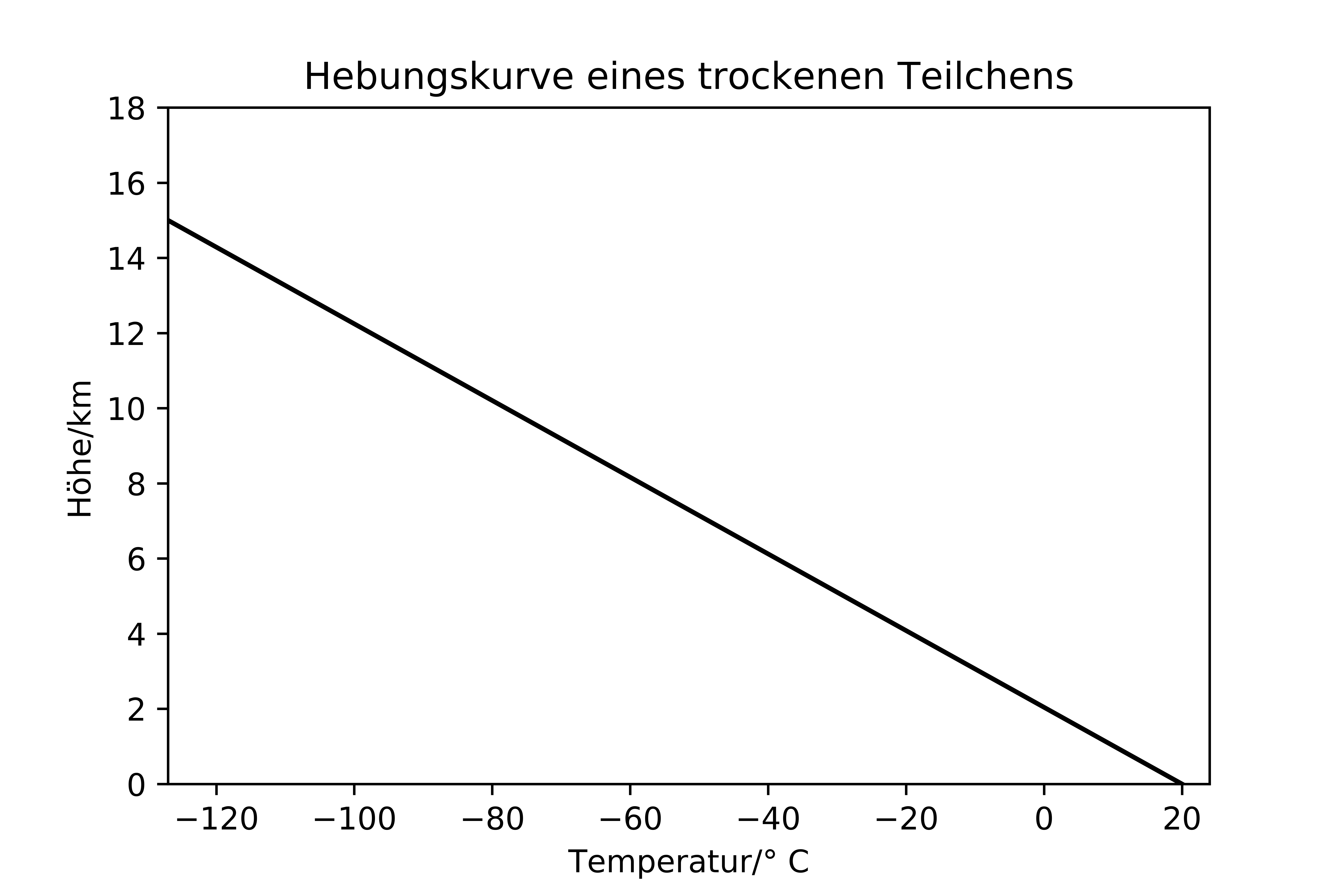
The dry adiabatic temperature gradient is not a temperature gradient in the true sense, it is the derivative of the function $T = T(z)$, which describes the adiabatic uplift of a particle. This function is also called dry adiabates. It is not the vertical component of the atmospheric temperature gradient $\nabla T$. This does not have to correspond at all, not even approximately, to the dry adiabatic. It is valid

\[ \begin{align} \frac{\partial T}{\partial z} &= \theta\frac{\partial p}{\partial z}\frac{R_s}{c^{(p)}}\frac{1}{p_0}\left(\frac{p}{p_0}\right)^{\frac{R_s}{c^{(p)}} - 1} + \frac{\partial\theta}{\partial z}\left(\frac{p}{p_0}\right)^{\frac{R_s}{c^{(p)}}} = -\frac{g}{c^{(p)}} - g\frac{p}{R_sT}\frac{\partial\theta}{\partial p}\left(\frac{p}{p_0}\right)^{\frac{R_s}{c^{(p)}}}\nonumber\\ \Rightarrow g\frac{p}{R_s\theta}\frac{\partial\theta}{\partial p} &= -\left(\Gamma_d - \Gamma\right)\tag{9.48}\label{eq:vert_temp_gradient} \end{align} \]

with

\[ \begin{align} \Gamma \coloneqq -\frac{\partial T}{\partial z}. \end{align} \]

The material derivation of Eq. (9.43) is

\[ \begin{align} \md{T} &= \md{\theta}\left(\frac{p}{p_0}\right)^{R_s/c^{(p)}} + \theta\frac{dp}{dt}\frac{1}{p_0}\frac{R_s}{c^{(p)}}\left(\frac{p}{p_0}\right)^{R_s/c^{(p)} - 1} = \frac{T}{\theta}\md{\theta} + \frac{T}{p}\omega\frac{R_s}{c^{(p)}} = \frac{T}{\theta}\md{\theta} + \frac{\omega}{\rho c^{(p)}}. \end{align} \]

From this it follows

\[ \begin{align} c^{(V)}\frac{T}{\theta}\md{\theta} + \frac{T}{p}\omega\frac{R_s}{c^{(p)}}c^{(V)} + p\md{}\frac{R_sT}{p} &= \frac{q_T^{(V)}}{\rho} - \frac{sT}{\rho}q_\rho^{(V)}\nonumber\\ \Leftrightarrow \md{\theta}\frac{T}{\theta} + \frac{\omega T}{p}\frac{R_s}{c^{(p)}} - \frac{R_sT}{pc^{(V)}}\omega + \frac{R_s}{c^{(V)}}\md{T} &= \frac{q_T^{(V)}}{c^{(V)}\rho} - \frac{sT}{c^{(V)}\rho}q_\rho^{(V)}\nonumber\\ \Leftrightarrow \frac{T}{\theta}\md{\theta} + \frac{\omega R_sT}{p}\left(\frac{1}{c^{(p)}} - \frac{1}{c^{(V)}}\right)\nonumber\\ + \frac{R_s}{c^{(V)}}\left(\frac{T}{\theta}\md{\theta} + \frac{T}{p}\omega\frac{R_s}{c^{(p)}}\right) &= \frac{q_T^{(V)}}{c^{(V)}\rho} - \frac{sT}{c^{(V)}\rho}q_\rho^{(V)}\nonumber\\ \Leftrightarrow \frac{T}{\theta}\md{\theta}\frac{c^{(p)}}{c^{(V)}} + \frac{\omega R_sT}{p}\frac{c^{(V)} - c^{(p)} + R_s}{c^{(V)}c^{(p)}} &= \frac{q_T^{(V)}}{c^{(V)}\rho} - \frac{sT}{c^{(V)}\rho}q_\rho^{(V)}. \end{align} \]

This means that the first law of thermodynamics for a gas reads in terms of potential temperature

Multiplying this equation by $\rho$ gives

\[ \begin{align} \rho\frac{\partial\theta}{\partial t} + \rho\mathbf{v}\cdot\nabla\theta = \frac{\theta}{Tc^{(p)}}\left(q_T^{(V)} - sTq_\rho^{(V)}\right). \end{align} \]

Add the product of the potential temperature with the continuity equation

\[ \begin{align} \theta\frac{\partial\rho}{\partial t} + \theta\mathbf{v}\cdot\nabla\rho + \theta\rho\nabla\cdot\mathbf{v} = \theta q_\rho^{(V)} = \frac{\theta}{Tc^{(p)}}Tc^{(p)}q_\rho^{(V)} \end{align} \]

added, follows

This form is also referred to as flow form, whereas Eq. (9.52) advection form. The flow form can be understood as a formal continuity equation.

9.2 The isentropic dry atmosphere

In an isentropic atmosphere (atmosphere of homogeneous specific entropy), according to Eq. (9.30) the potential temperature is also homogeneous. This leads to a different dependence of pressure on altitude than in the case of the isothermal atmosphere. If $\Gamma_d > 0$ is the dry adiabatic temperature gradient, the temperature is $T(z) = T_0 - \Gamma_d z$ with $T_0 \coloneqq T(z = 0)$. This follows

\[ \begin{align} \frac{\partial p}{\partial z} = -g\rho = -g\frac{p}{R_dT} = -\frac{g}{R_d}\frac{p}{T_0 - \Gamma_d z} = \frac{gp}{R_d(\Gamma_d z - T_0)} \end{align} \]

as a differential equation to be solved for $p = p(z)$. You do the approach

\[ \begin{align} p(z) = C\exp\left[f(z)\right] \end{align} \]

with a continuously differentiable function $f = f(z)$ and a constant $C > 0$, it follows

\[ \begin{align} \frac{\partial p}{\partial z} = \frac{\partial f}{\partial z}p, \end{align} \]

so you get for $f$

\[ \begin{align} \frac{\partial f}{\partial z} = \frac{g}{R_d\left(\Gamma_d z - T_0\right)}, \end{align} \]

this is solved for

\[ \begin{align} f = \frac{g}{R_d\Gamma_d}\ln\left(T_0 - \Gamma_d z\right). \end{align} \]

This follows for printing

\[ \begin{align} p(z) = C\exp\left(\frac{g}{R_d\Gamma_d}\ln\left(T_0 - \Gamma_d z\right)\right) = C\left(T_0 - \Gamma_d z\right)^{\frac{g}{R_d\Gamma_d}}, \end{align} \]

with $p(0) = p_0$ it follows $C = \frac{p_0}{T_0^{\frac{g}{\Gamma_d R_d}}}$. So it applies

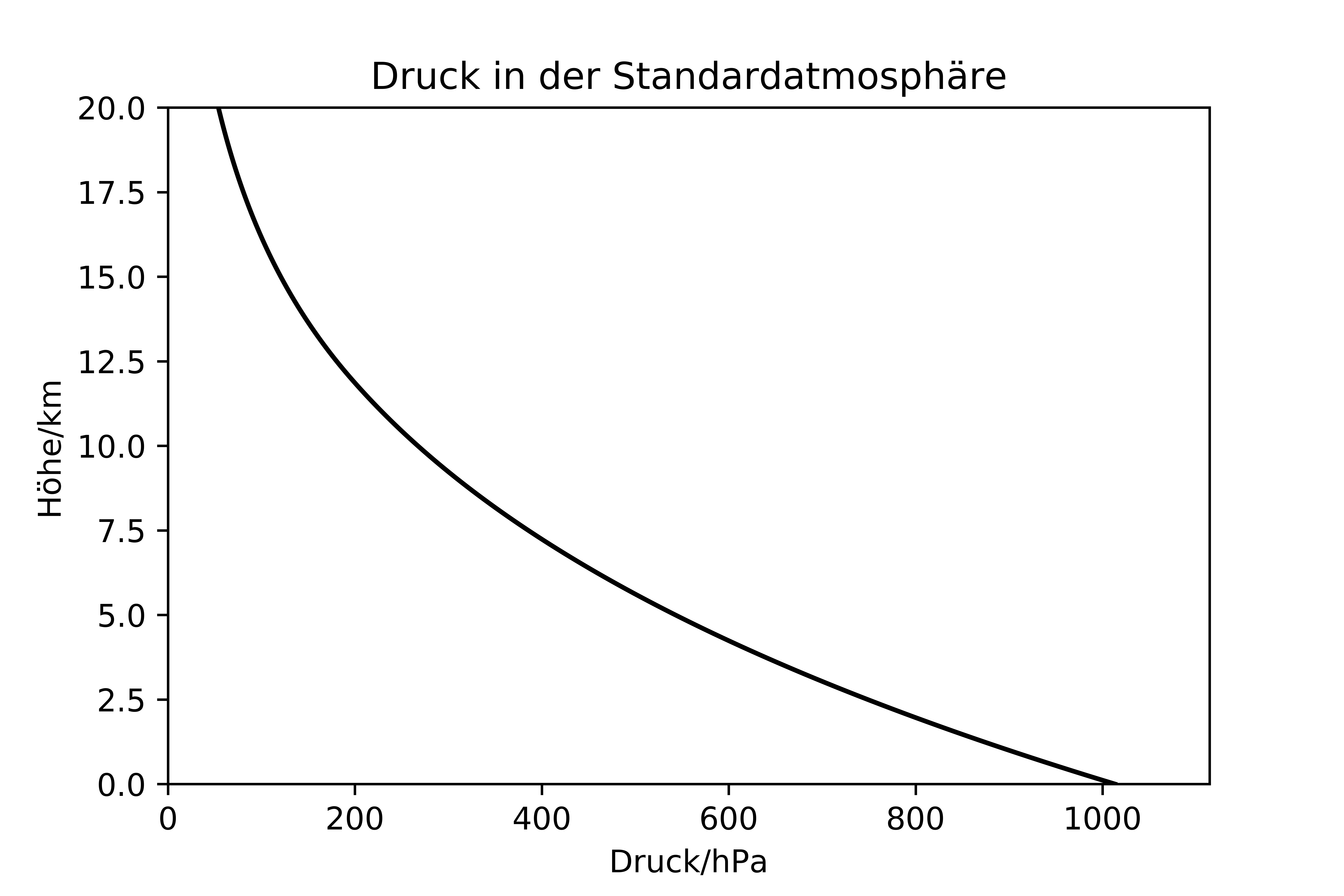
In the troposphere, a linear decrease in temperature with altitude is more realistic than isothermia. However, the dry adiabatic gradient is climatologically too extreme. The standard atmosphere is assumed to be an atmosphere with a temperature of $T_0 = 290$ K $ = 16.85^\circ$ C reduced to the geopotential surface zero and a linear temperature decrease $k = 0.65$ K/100m up to an altitude $H = 12$ km. This is assumed to be isothermal. If you replace the dry adiabatic gradient $\Gamma_d$ by $k$ in the formula for the isentropic atmosphere (9.62) and use the barometric altitude formula above it, it follows

\[ \begin{align} p(z) &= \left\lbrace\begin{array}{c} p_0\left(1 - \frac{kz}{T_0}\right)^\frac{g}{R_dk}, \:z < H\\ p(H)\exp\left(-g\frac{z - H}{R_dT_T}\right) , \:z\geq H \end{array}\right. \end{align} \]

with $T_T \coloneqq T_0 - kH$ as the temperature of the tropopause.

In a stable atmosphere, $\theta$ is a possible vertical coordinate, one speaks of isentropic coordinates, since the surfaces with the same vertical coordinate are surfaces with the same entropy.

9.3 Further forms of the first law in the atmosphere

9.3.1 Pressure as a prognostic variable

Now the definition of the potential temperature should be inserted into the equation of state:

\[ \begin{align} p &= \rho R_s\theta\left(\frac{p}{p_0}\right)^{R_s/c^{(p)}}\Rightarrow p^{1 - R_s/c^{(p)}} = \rho R_s\theta\frac{1}{p_0^{R_s/c^{(p)}}}\tag{9.64}\label{eq:state_theta_deriv_0}\\ \Rightarrow p^{1/\kappa} &= \rho R_s\theta\frac{1}{p_0^{R_s/c^{(p)}}}\Rightarrow p = \left(\rho R_s\theta\right)^\kappa\left(\frac{1}{p_0}\right)^{\kappa - 1}\tag{9.65}\label{eq:state_theta} \end{align} \]

A prognostic equation can also be derived for $p$:

\[ \begin{align} p &= \rho R_sT \Rightarrow \md{p} = R_s\left(T\md{\rho} + \rho\md{T}\right) \end{align} \]

With

\[ \begin{align} \md{\rho} = -\rho\nabla\cdot\mathbf{v} + q_\rho^{(V)}, & {} & \md{T} = \frac{T}{\theta}\md{\theta} + \frac{TR_s}{c^{(p)}p}\md{p} \end{align} \]

follows

\[ \begin{align} \md{p} &= R_sT\left(-\rho\nabla\cdot\mathbf{v} + q_{\rho}\right) + R_s\rho\left(\frac{T}{\theta}\md{\theta} + \frac{TR_s}{c^{(p)}p}\md{p}\right)\nonumber\\ &= -p\nabla\cdot\mathbf{v} + R_sTq_\rho^{(V)} + \frac{p}{\theta}\md{\theta} + \frac{R_s}{c^{(p)}}\md{p}\nonumber\\ \Leftrightarrow \frac{c^{(V)}}{c^{(p)}}\md{p} &= -p\nabla\cdot\mathbf{v} + R_sTq_\rho^{(V)} + \frac{p}{\theta}\md{\theta}\nonumber\\ \Leftrightarrow \frac{\partial p}{\partial t} &= -\mathbf{v}\cdot\nabla p - \frac{c^{(p)}}{c^{(V)}}p\nabla\cdot\mathbf{v} + \frac{c^{(p)}}{c^{(V)}}R_sTq_\rho^{(V)} + \frac{p}{T\rho c^{(V)}}\left(q_T^{(V)} - sTq_\rho^{(V)}\right) \end{align} \]

9.3.2 Exner pressure as a prognostic variable

Define the Exner pressure $\Pi$ by

\[ \begin{align} \Pi \coloneqq \frac{T}{\theta} = \left(\frac{p}{p_0}\right)^{R_s/c^{(p)}} \Leftrightarrow p = \Pi^{c^{(p)}/R_s}p_0,\tag{9.70}\label{eq:def_exner-druck} \end{align} \]

the connection applies

\[ \begin{align} p &= \rho R_s\theta\Pi \Leftrightarrow \Pi^{c^{(p)}/R_s} = \frac{\rho R_s\theta}{p_0}\Pi \Leftrightarrow \Pi^{c^{(V)}/R_s} = \frac{\rho R_s\theta}{p_0}\nonumber\\ \Leftrightarrow\Pi &= \left(\frac{\rho R_s\theta}{p_0}\right)^{R_s/c^{(V)}}.\tag{9.71}\label{eq:exner_pressure_diag} \end{align} \]

From this it follows

\[ \begin{align} \nabla p = R_s \theta\rho\nabla\Pi + R_s\Pi\nabla\left(\rho\theta\right) = c^{(p)}\theta\rho\nabla\Pi - c^{(V)}\theta\rho\nabla\Pi + R_s\Pi\nabla\left(\rho\theta\right). \end{align} \]

One finds:

\[ \begin{align} -c^{(V)}\theta\rho\nabla\Pi + R_s\Pi\nabla\left(\rho\theta\right) &= -\left(\frac{R_s}{p_0}\right)^{R_s/c^{(V)}}c^{(V)}\theta\rho\nabla\left(\rho\theta\right)^{R_s/c^{(V)}} + R_s\Pi\nabla\left(\rho\theta\right)\nonumber\\ &\stackrel{\text{Glg. }\href{#eq:exner_pressure_diag}{(9.71)}}{=} R_s\left(\Pi - \left(\frac{R_s}{p_0}\right)^{R_s/c^{(V)}}\left(\rho\theta\right)^{R_s/c^{(V)}}\right)\nabla\left(\rho\theta\right) = 0 \end{align} \]

So you can write for the pressure gradient acceleration

\[ \begin{align} -\frac{1}{\rho}\nabla p = -c^{(p)}\theta\nabla\Pi.\tag{9.74}\label{eq:exner_pressure_gradient_acc} \end{align} \]

With Eq. (B.49) follows

\[ \begin{align} \nabla\cdot\left(\rho c^{(p)}\Pi\theta\mathbf{v}\right) &= \rho c^{(p)}\theta\mathbf{v}\cdot\nabla\Pi + \Pi\nabla\cdot\left(\rho c^{(p)}\theta\mathbf{v}\right)\nonumber\\ \Leftrightarrow -\rho\mathbf{v}\cdot c^{(p)}\theta\nabla\Pi &= -\nabla\cdot\left(\rho c^{(p)}T\mathbf{v}\right) + c^{(p)}\Pi\nabla\cdot\left(\rho\theta\mathbf{v}\right)\nonumber\\ \Leftrightarrow -\rho\mathbf{v}\cdot c^{(p)}\theta\nabla\Pi &= -\nabla\cdot\left(\rho h\mathbf{v}\right) + c^{(p)}\Pi\nabla\cdot\left(\rho\theta\mathbf{v}\right)\ \end{align} \]

with the specific enthalpy $h$. From this you can deduce:

• If the pressure gradient has an accelerating effect, the flow of potential temperature diverges more than the flow of enthalpy.
• If the pressure gradient has a braking effect, the flow of enthalpy diverges more than the flow of potential temperature.

Now two more prognostic equations for $\Pi$ are derived. The local time derivation of Eq. (9.71) is in the adiabatic case

\[ \begin{align} \frac{\partial\Pi}{\partial t} &= \frac{R_s}{c^{(V)}}\left(\frac{\rho R_s\theta}{p_0}\right)^{\frac{R_s}{c^{(V)}} - 1}\frac{\rho R_s\theta}{p_0}\left(\frac{1}{\theta}\frac{\partial\theta}{\partial t} + \frac{1}{\rho}\frac{\partial\rho}{\partial t}\right) = \frac{R_s}{c^{(V)}\theta\rho}\left(\frac{\rho R_s\theta}{p_0}\right)^{\frac{R_s}{c^{(V)}}}\left(\rho\frac{\partial\theta}{\partial t} + \theta\frac{\partial\rho}{\partial t}\right)\nonumber\\ &= \frac{R_s\Pi}{c^{(V)}\theta\rho}\left(\rho\frac{\partial\theta}{\partial t} + \theta\frac{\partial\rho}{\partial t}\right) = \frac{R_s\Pi}{c^{(V)}\theta\rho}\left(-\rho\mathbf{v}\cdot\nabla\theta - \theta\nabla\cdot\left(\rho\mathbf{v}\right)\right) = -\frac{R_s\Pi}{c^{(V)}\theta\rho}\nabla\cdot\left(\rho\theta\mathbf{v}\right). \end{align} \]

If you add the diabatic terms, it follows

For the material derivation of Eq. (9.71) is obtained

\[ \begin{align} \md{\Pi} = \frac{R_s}{c^{(V)}}\left(\frac{\rho R_s\theta}{p_0}\right)^{R_s/c^{(V)} - 1}\frac{R_s}{p_0}\md{\left(\rho\theta\right)} = \frac{R_s}{c^{(V)}\rho\theta}\left(\frac{\rho R_s\theta}{p_0}\right)^{R_s/c^{(V)}}\md{\left(\rho\theta\right)} = \frac{R_s\Pi}{c^{(V)}\rho\theta}\md{\left(\rho\theta\right)}. \end{align} \]

With Eq. (9.55) follows

9.4 Ideal gas mixture with a homogeneous composition

N-atomic ideal gases have additional rotational and vibrational degrees of freedom compared to monatomic gases. These additional degrees of freedom increase the heat capacities and an analytical expression for the entropy is then no longer available. A monatomic ideal gas with the same average molar mass as the original gas is used as a model for this complex system, with measured values ​​or products of a more fundamental theory used for the heat capacities. This means that the results listed in the previous section can also be transferred to dry air.

9.5 Ideal gas mixture with variable composition

Here we assume a gas mixture of $N \geq 1$ ideal monatomic gases. Eq. (9.34) can be applied and overlaid on any of these components. This applies

\[ \begin{align} \newtilde{s}_i = s_i\rho_i \end{align} \]

for $1 \leq i \leq N$ and

\[ \begin{align} s = \sum_{i = 1}^N\newtilde{s}_i. \end{align} \]

In principle, each type of gas gets its own temperature source term $q_{T, i}$. However, to simplify matters, it is assumed that the subsequent exchange of energy between the types of gas is so fast that it can be assumed to be instantaneous. In this case you can

\[ \begin{align} q_{T, i}^{(V)} = \frac{\rho_ic_i^{(V)}}{\sum_{j = 1}^N\rho_jc_j^{(V)}}q_T^{(V)} \end{align} \]

Therefore, Eq. (9.34)

also with these definitions.

9.5.1 Example: moist air

One defines the so-called virtual potential temperature

$\theta_v$ durch

\[ \begin{align} \theta_v \coloneqq T_v\left(\frac{p_0}{p}\right)^{R_d/c_d^{(p)}}, \end{align} \]

here is

\[ \begin{align} T_v = T\left[1 + \frac{\rho_v}{\rho_h}\left(\frac{M_d}{M_v} - 1\right)\right] \end{align} \]

those in Eq. (5.164) defined virtual temperature. The virtual potential temperature is not the potential temperature of moist air $\theta_h$, because for this would

\[ \begin{align} \theta_h \coloneqq T\left(\frac{p_0}{p}\right)^{R_h/c_h^{(p)}} \end{align} \]

apply. The virtual potential temperature is the potential temperature that dry air would have to have in order to have the same density after adiabatic compression to the reference pressure $p_0$ like the moist air under consideration.

For the specific isochoric heat capacity of moist air $c_h^{(v)}$ applies

\[ \begin{align} c_h^{(v)} = \frac{\rho_dc_d^{(v)} + \rho_vc_v^{(v)}}{\rho_d + \rho_v} = c_d^{(v)}\frac{\rho_d + \rho_v\frac{c_v^{(v)}}{c_d^{(v)}}}{\rho_d + \rho_v} = c_d^{(v)}\frac{\rho_h - \rho_v + \rho_v\frac{c_v^{(v)}}{c_d^{(v)}}}{\rho_h} = c_d^{(v)}\left[1 + \frac{\rho_v}{\rho_h}\left(\frac{c_v^{(v)}}{c_d^{(v)}} - 1\right)\right] \end{align} \]

According to Eq. (5.148) applies in ideal gas

\[ \begin{align} \frac{c_v^{(v)}}{c_d^{(v)}} = \frac{M_d}{M_v}. \end{align} \]

However, if you insert the actual values, you get

\[ \begin{align} \frac{c_v^{(v)}}{c_d^{(v)}} = 1,945 \not= 1,608 = \frac{M_d}{M_v}.\tag{9.89}\label{eq:theta_v_not_accurate} \end{align} \]

This shows that although real gases can be described very well under atmospheric conditions by the thermal equation of state of ideal gases, their material properties cannot. However, if you ignore this deviation, it follows

\[ \begin{align} c_h^{(v)} = c_d^{(v)}\left[1 + \frac{\rho_v}{\rho_h}\left(\frac{M_d}{M_v} - 1\right)\right] \end{align} \]

The adiabatic form of the first law of thermodynamics Eq. (9.14) can now be formulated in virtual temperature terms:

\[ \begin{align} c_h^{(v)}\md{T} + R_hT\nabla\cdot\mathbf{v} &= 0\nonumber\\ \Leftrightarrow c_d^{(v)}\left[1 + \frac{\rho_v}{\rho_h}\left(\frac{M_d}{M_v} - 1\right)\right]\md{T} + R_dT_v\nabla\cdot\mathbf{v} &= 0\nonumber\\ \Leftrightarrow c_d^{(v)}\md{\left\lbrace T\left[1 + \frac{\rho_v}{\rho_h}\left(\frac{M_d}{M_v} - 1\right)\right]\right\rbrace} + R_dT_v\nabla\cdot\mathbf{v} &= 0\nonumber\\ \Leftrightarrow c_d^{(v)}\md{T_v} + R_dT_v\nabla\cdot\mathbf{v} &= 0 \end{align} \]

The prefactor $1 + \frac{\rho_v}{\rho_h}\left(\frac{M_d}{M_v} - 1\right)$, which turns the temperature into the virtual temperature, can be included in the derivation, since the term $\propto \md{q}$ resulting from the product rule according to Eq. (7.28) is equal to zero for adiabatic processes. In humid air you can use adiabatic processes to replace the equations for dry air

\[ \begin{align} T \to T_v \end{align} \]

use if the inaccuracy according to Inq. (9.89) accepted.

9.6 Thermodynamic significance of heat conduction

Eq. (9.83)

\[ \begin{align} \frac{\partial\newtilde{s}}{\partial t} + \nabla\cdot\left(\newtilde{s}\mathbf{v}\right) &= \frac{q_T^{(V)}}{T}\tag{9.93}\label{eq:td_1_2_entropy_id_gas_repeat} \end{align} \]

is a combination of the first and second laws of thermodynamics. For $q_T^{(V)}$ applies in the absence of radiation and condensates

\[ \begin{align} q_T^{(V)} = -\nabla\cdot\mathbf{j}_q + \epsilon, \end{align} \]

here $\mathbf{j}_q$ is the heat flux density through heat conduction. According to Eq. (5.219) applies

\[ \begin{align} \mathbf{j}_q = -\rho c_d^{(v)}\kappa\nabla T. \end{align} \]

You can now do the math

\[ \begin{align} \frac{\nabla\cdot\left(\rho\kappa\nabla T\right)}{T} = \nabla\cdot\frac{\rho c_d^{(v)}\kappa\nabla T}{T} + \frac{\rho c_d^{(v)}\kappa}{T^2}\left(\nabla T\right)^2 = -\nabla\cdot\frac{\mathbf{j}_q}{T} + \frac{\rho c_d^{(v)}\kappa}{T^2}\left(\nabla T\right)^2. \end{align} \]

Putting this into Eq. (9.93) and integrate globally, you get

\[ \begin{align} \int_A\frac{\partial\newtilde{s}}{\partial t}d^3r &= \frac{d}{dt}\int_A\newtilde{s}d^3r = \int_A-\nabla\cdot\frac{\mathbf{j}_q}{T} + \frac{\rho c_d^{(v)}\kappa}{T^2}\left(\nabla T\right)^2d^3r = -\int_{\partial A}\frac{\mathbf{j}_q}{T}\cdot d\mathbf{n} + \int_A\frac{\rho c_d^{(v)}\kappa}{T^2}\left(\nabla T\right)^2d^3r. \end{align} \]

The evolution equation of the total entropy of the atmosphere

\[ \begin{align} S = \int_A\newtilde{s}d^3r \end{align} \]

in this case is:

Internal processes in an ideal gas with viscosity can therefore only produce entropy, as required by the second law of thermodynamics.

9.7 Condensates

The first law must also be formulated for the condensate classes $i$. To do this, one starts from Eq. (5.34) from:

\[ \begin{align} \Delta U_i = \Delta Q_i - \Delta W_i \end{align} \]

The condensates are assumed to be incompressible, i.e. $\Delta W_i = 0$. In addition to radiation, heat transfer and dissipation, phase transitions also play a role as heat sources. These work in two ways:

• They lead to latent heat flows and thus change the temperature.
• They change the composition of the components of the air and change the temperature through mixing.

The first point is discussed in Chap. 11 described in more detail. All heat flows that act on phase $i$ per volume are combined into a source strength $q_i$. This is about the second point, i.e. the effect of mass flows on the temperature $T_i$ is to be examined. Eq. (7.25) includes five types of mass fluxes, viz

• Phase transitions in which new condensate particles are formed,
• Phase transitions that take place on the surface of a particle,
• Phase transformations of condensate particles so that they change their class,
• collisions and
• Decay processes

Only processes in which matter transitions into phase $i$ contribute to a change in temperature $T_i$. The class $i$ has the specific heat capacity $c_i$, the $m_j$ and $m_h$ are the masses passing into the phase $i$. Then applies to the heat content before or after a mass flow

\[ \begin{align} c_im_iT_i\left(t\right) + c_hm_hT + \sum_{j\not = i}^{}c_jm_jT_j &= c_iT_i\left(t + \Delta t\right)\left(m_h + m_i + \sum_{j\not = i}^{}m_j\right)\nonumber\\ \Leftrightarrow c_im_i\left[T_i\left(t + \Delta t\right) - T_i\left(t\right)\right] &= c_hm_hT + \sum_{j\not = i}^{}c_jm_jT_j - c_iT_i\left(t + \Delta t\right)\left(m_h + \sum_{j\not = i}^{}m_j\right)\nonumber\\ \Leftrightarrow\Delta T_i &= \frac{c_h}{c_im_i}m_h\left(T - \frac{c_i}{c_h}T_i\left(t + \Delta t\right)\right) + \frac{1}{c_im_i}\sum_{j\not = i}\left[c_jm_jT_j - c_im_jT_i\left(t + \Delta t\right)\right]\nonumber\\ \Leftrightarrow \frac{1}{\Delta V}\frac{dT_i}{dt} &= \frac{1}{m_i}\newtilde{q}_{hi}\left(\frac{c_h}{c_i}T - T_i\right) + \frac{1}{m_i}\sum_{j\not = i}^{}\newtilde{q}_{j, i}\left(\frac{c_j}{c_i}T_j - T_i\right)\nonumber\\ \Leftrightarrow\rho_ic_i\frac{dT_i}{dt} &= \newtilde{q}_{hi}\left(c_hT - c_iT_i\right) + \sum_{j}^{}\newtilde{q}_{j, i}\left(c_jT_j - c_iT_i\right). \end{align} \]

It was assumed that all particles of class $i$ have the same temperature $T_i$, meaning that instantaneous mixing occurs. According to Eq. (7.25) and the considerations in section 11.2 apply

\[ \begin{align} \newtilde{q}_{hi} = \newtilde{q}_{v, i}' + \newtilde{q}_{v, i}''. \end{align} \]

Phase transformations, collisions and decay processes contribute to the $\newtilde{q}_{j, i}$. According to the considerations in the derivation of Eq. (7.25) applies

\[ \begin{align} \newtilde{q}_{j, i} = \newtilde{m}_j\sum_{k}^{}\sigma_{j, k}n_jn_k\newoverline{v_{\text{rel}}}\left(j, k\right)P_{j, k}\delta_{i, R_{j, k}} + \newtilde{m}_i\lambda_jn_j\sum_l\left(Z_{jil}\right) + \newtilde{q}_{j, i}'''. \end{align} \]

So you have

The notation explicitly takes into account that what is meant is the isochoric specific heat capacity. An analogous term must also be taken into account for moist air: