16 Waves and instabilities

The equations of motion have wave solutions. These are obtained by inserting a complex harmonic ansatz $\mathbf{\psi}_0e^{-i\omega t}$ into the respective system of equations and seeking non-trivial solutions; here $\mathbf{\psi}_0$ is a complex amplitude vector. Occasionally, a zonal background current is included because of its climatological relevance. A solution is an instability if $\Im\left(\omega\right) > 0$, i.e. if the amplitude grows exponentially.

16.1 Kinematics

Waves are periodic changes in space and time. The maximum absolute deflection from the rest position is the amplitude. The time $T > 0$ until the motion pattern repeats at a fixed location is called the period; its inverse is the frequency $f$. The angular frequency $\omega$ is defined as

\[ \begin{align} \omega \coloneqq 2\pi f = \frac{2\pi}{T}. \end{align} \]

Analogously, the wavelength $\lambda > 0$ is the length after which the motion pattern repeats. The wavenumber $\kappa$ and the angular wavenumber $k$ are defined analogously to the frequency and angular frequency by

\[ \begin{align} \kappa \coloneqq \frac{1}{\lambda}, & {} & k \coloneqq \frac{2\pi}{\lambda}. \end{align} \]

A wave in a quantity $a$ is described by an equation of the form

\[ \begin{align} a\left(x, t\right) = Af\left(kx - \omega t + \varphi\right). \end{align} \]

Here $f$ is a real- or complex-valued, $2\pi$-periodic function, i.e. $f\left(\xi + 2\pi\right) = f\left(\xi\right)$ for each $\xi\in \mathbb{R}$. It need not be trigonometric. $f$ is often chosen to be complex-valued, e.g. $f(x) = \exp(ix)$, if this makes the notation shorter or clearer. Before comparing with measured quantities, however, the result must be projected onto the real axis. The argument $kx - \omega t + \varphi$ is called the phase of the wave; in the complex plane, this is the angle with the real axis. The parameter $\varphi$ is a phase shift, allowing a nonzero phase at $x=t=0$. In derivations, $\varphi$ can often be removed by shifting the time or spatial coordinates. The quantities $k$ and $\omega$ may also have imaginary parts, e.g. for waves that decay exponentially into a medium (so-called evanescent waves) or for instabilities with exponentially growing amplitude. Likewise, the prefactor $A$ may be complex and therefore include a phase shift.

In general, a wave can also propagate in a three-dimensional space, in which case one first writes in general terms

\[ \begin{align} a\left(\mathbf{r}, t\right) = Af\left(\phi\left(\mathbf{r}, t\right)\right) \end{align} \]

with $\phi = \phi\left(\mathbf{r}, t\right)$ the phase function. The phase function can, for example, have the form

\[ \begin{align} \varphi\left(\mathbf{r}, t\right) = \mathbf{k}\cdot\mathbf{r} - \omega t\tag{16.5}\label{eq:phase_velocity_deriv} \end{align} \]

here $\mathbf{k} = \left(k_x, k_y, k_z\right)^T$ is called the wave vector. Its magnitude equals the angular wavenumber, and it points in the direction of propagation of the wave. Differentiating Eq. (16.5) with respect to time yields

\[ \begin{align} \frac{d\varphi\left(\mathbf{r}, t\right)}{dt} = \mathbf{k}\cdot\frac{d\mathbf{r}}{dt} - \omega \end{align} \]

Setting the left-hand side equal to zero—i.e. moving with a point of constant phase—and choosing a trajectory parallel to $\mathbf{k}$, one obtains the phase velocity

The dependence

\[ \begin{align} \omega = \omega\left(k\right) \end{align} \]

is called the dispersion relation. Now consider the superposition $f\left(x, t\right) = f_1\left(x, t\right) + f_2\left(x, t\right)$ of two waves:

\[ \begin{align} f_1\left(x, t\right) &= -\cos\left(k_1x - \omega_1t\right)\\ f_1\left(x, t\right) &= \cos\left(k_2x - \omega_2t\right)\\ f\left(x, t\right) &= -\cos\left(k_1x - \omega_1t\right) + \cos\left(k_2x - \omega_2t\right) \end{align} \]

With Eq. (A.63), it follows that

\[ \begin{align} -\cos\left(\alpha\right) + \cos\left(\beta\right) &= 1 - \cos\left(\alpha\right) - 1 + \cos\left(\beta\right) = 2\sin^2\left(\frac{\alpha}{2}\right) - 2\sin^2\left(\frac{\beta}{2}\right)\nonumber\\ &= 2\sin^2\left(\frac{\alpha}{2}\right) - 2\sin^2\left(\frac{\alpha}{2}\right)\sin^2\left(\frac{\beta}{2}\right) - 2\sin^2\left(\frac{\beta}{2}\right) + 2\sin^2\left(\frac{\alpha}{2}\right)\sin^2\left(\frac{\beta}{2}\right)\nonumber\\ &= 2\left[\sin^2\left(\frac{\alpha}{2}\right)\cos^2\left(\frac{\beta}{2}\right) - \cos^2\left(\frac{\alpha}{2}\right)\sin^2\left(\frac{\beta}{2}\right)\right]\nonumber\\ &= 2\left[\sin\left(\frac{\alpha}{2}\right)\cos\left(\frac{\beta}{2}\right) - \cos\left(\frac{\alpha}{2}\right)\sin\left(\frac{\beta}{2}\right)\right]\left[\sin\left(\frac{\alpha}{2}\right)\cos\left(\frac{\beta}{2}\right) + \cos\left(\frac{\alpha}{2}\right)\sin\left(\frac{\beta}{2}\right)\right]\nonumber\\ &= 2\sin\left(\frac{\alpha - \beta}{2}\right)\sin\left(\frac{\alpha + \beta}{2}\right). \end{align} \]

Thus,

\[ \begin{align} f\left(x, t\right) &= 2\sin\left(\frac{\Delta k x - \Delta\omega t}{2}\right)\sin\left(\newoverline{k}x - \newoverline{\omega}t\right) \end{align} \]

with

\[ \begin{align} \Delta k \coloneqq k_2 - k_1, & {} & \Delta\omega \coloneqq \omega_2 - \omega_1,\\ \newoverline{k} \coloneqq \frac{k_1 + k_2}{2}, & {} & \newoverline{\omega} \coloneqq \frac{\omega_1 + \omega_2}{2}. \end{align} \]

The envelope $\sin\left(\frac{\Delta k x - \Delta\omega t}{2}\right)$ thus moves with the velocity

\[ \begin{align} v_e = \frac{\Delta\omega}{\Delta k}. \end{align} \]

One therefore defines the group velocity $c_{\text{gr}}$ by

\[ \begin{align} c_{\text{gr}} \coloneqq \frac{\partial\omega}{\partial k}. \end{align} \]

It can therefore be derived from the dispersion relation. It is the velocity at which wave packets move, i.e. at which energy is transported. If

\[ \begin{align} c_{\text{gr}} = c \end{align} \]

independently of $k$, the wave is called dispersion-free. One can generalize the group velocity to the vector form

With $\omega = ck$, one can write

\[ \begin{align} c_{\text{gr}} &= \frac{d\omega}{dk} = c + k\frac{dc}{dk} = c + k\frac{d\lambda}{dk}\frac{dc}{d\lambda} = c - \frac{2\pi}{k}\frac{dc}{dy} = c - \lambda\frac{dc}{d\lambda}. \end{align} \]

In the case $dc/d\lambda < 0$ one speaks of abnormal dispersion. In this case the energy propagates faster than the phase velocity. In the case

\[ \begin{align} \frac{dc}{d\lambda}\lambda > c \Leftrightarrow \frac{dc}{d\lambda} > \frac{c}{\lambda} = f \end{align} \]

or

\[ \begin{align} \frac{d\omega}{dk} < 0 \end{align} \]

the energy propagates in a direction opposite to the wave vector.

If the character of a wave allows this, it is categorized either as a longitudinal wave, in which the oscillators oscillate parallel to the wave vector, or as a transverse wave, in which they oscillate perpendicular to it. For mechanical transverse waves, one introduces as further kinematic quantities the wave height $H$, equal to twice the amplitude, and the steepness $S$ of a wave, which is defined by

\[ \begin{align} S \coloneqq \frac{H}{\lambda} \end{align} \]

and is therefore dimensionless.

16.2 Categorization of waves in geofluids

Barotropic waves (see Sect. 16.5) require boundary surfaces and have their amplitude maximum at these. Therefore they are also referred to as external waves or surface waves. The shallow water equations are usually sufficient to describe such waves.

Baroclinic waves (see Sect. 16.6), however, exist inside a medium; they are therefore also referred to as internal waves.

A limiting case here are waves at a sharp interface ($N \gg 0$) inside a medium, such as at an inversion or a density jump (see, for example, the illustration at the end of Sect. 16.5.2). They can often be described mathematically using the formulas for surface waves, but are usually classified as internal waves. Capillary waves (see Sect. 16.4) are surface waves, but barotropy plays no role and the shallow water equations are not sufficient to describe them. Therefore they represent a special category.

16.3 Justification for linearization

If $A, B$ are two phenomena and $f\left(A + B\right)$ is, for example, a prediction, then in general it holds

\[ \begin{align} f\left(A + B\right) \not = f\left(A\right) + f\left(B\right), \end{align} \]

The total effect of $A + B$ is therefore not the sum of the individual effects $A, B$, since $f$ is not a linear map.

However, when searching for analytical solutions to a nonlinear system of equations, especially when searching for wave solutions, one is very interested in linearization. This is sometimes more, sometimes less justified. It is assumed that for a quantity $A = A_0 + A'$, with $A_0$ the background state and $A'$ the perturbation, one has

\[ \begin{align} \mathcal{O}\left(A_0\right) = \mathcal{O}\left(A'\right) + 1, \end{align} \]

and therefore

\[ \begin{align} \mathcal{O}\left(A'^2\right) = \mathcal{O}\left(A_0\right) - 2. \end{align} \]

One therefore neglects all terms in which products of the perturbations occur. This leads to a linearization of the system of equations. For the derivatives, assuming a plane wave in the x-direction with angular frequency $\omega$ and angular wavenumber $k$ that affects only the perturbations, one has

\[ \begin{align} \mathcal{O}\left(\frac{\partial A'}{\partial t}\right) &= \mathcal{O}\left(\omega A'\right),\\ \mathcal{O}\left(\frac{\partial A'}{\partial x}\right) &= \mathcal{O}\left(kA'\right)\\ \mathcal{O}\left(\frac{\frac{\partial A'}{\partial t}}{A\frac{\partial A'}{\partial x}}\right) &= \mathcal{O}\left(\frac{\omega}{Ak}\right) = \mathcal{O}\left(\frac{c}{A}\right).\tag{16.29}\label{eq:bed_lin_wellglg} \end{align} \]

From Eq. (16.29) it follows that one can neglect the advective terms if the phase velocity $c = \frac{\omega}{k}$ is much larger than the fluid particle velocity.

If it is possible to eliminate all nonlinear terms of a system of equations, then one knows that two independent solutions to this system of equations do not affect each other. Examples are sound waves and electromagnetic waves. The linearity of these systems makes it possible to independently superimpose different sounds or signals.

16.3.1 Example: sound waves

Sound waves are compression waves; however, because of the adiabatic nature of the process, pressures and densities can be uniquely mapped onto one another. A wave propagating in the x direction is considered. The perturbation ansatz for velocity and density is

\[ \begin{align} u = U + u', & {} & \rho = \rho_0 + \rho'. \end{align} \]

The system of equations, with the abbreviating replacements

\[ \begin{align} \rho' &\to \rho,\\ u' &\to u \end{align} \]

and the approximations derived in the previous section, thus reads

\[ \begin{align} \frac{\partial u}{\partial t} + U\frac{\partial u}{\partial x} &= -\frac{1}{\rho _0}\frac{\partial p}{\partial x}\tag{16.33}\label{eq:schall_1}\\ \frac{\partial\rho}{\partial t} + U\frac{\partial \rho}{\partial x} &= - \rho _0\frac{\partial u}{\partial x}\tag{16.34}\label{eq:schall_2}\\ \rho(p) &= \rho_\theta\left(\frac{p}{p_0}\right)^{c_v/c_p} \end{align} \]

The first equation is the momentum equation, the second is the continuity equation, and the third is the potential density equation Eq. (9.44). In order to express the change in density through the pressure in Eq. (16.34), one uses the chain rule:

\[ \begin{align} \frac{\partial\rho}{\partial t} = \frac{\partial\rho}{\partial p}\frac{\partial p}{\partial t} = \frac{\rho_\theta c_v}{p_0c_p}\left(\frac{p}{p_0}\right)^{c_v/c_p - 1}\frac{\partial p}{\partial t} = \frac{\rho_\theta c_v}{p_0c_p}\frac{\partial p}{\partial t}, \end{align} \]

analogously for $\frac{\partial}{\partial x}$. The derivative of the density with respect to the pressure was evaluated at $p = p_0$, because the pressure fluctuations are very small. Now one makes the ansatz

\[ \begin{align} u = u_0\exp\left[i\left(kx - \omega t\right)\right], & {} & p = P\exp\left[i\left(kx - \omega t\right)\right] \end{align} \]

with possibly complex amplitudes $u_0, P$. Substituting this into the system of equations, one obtains

\[ \begin{align} -i\omega u_0 + Uiku_0 &= -\frac{1}{\rho_\theta}ikP,\\ -\frac{\rho_\theta c_v}{p_0c_p}i\omega P + Uik\frac{\rho_\theta c_v}{p_0c_p}P &= -\rho_\theta iku_0\nonumber\\ \Leftrightarrow - i\omega P + UikP &= -\frac{p_0c_p}{c_v}iku_0. \end{align} \]

As a matrix equation this becomes

\[ \begin{align} \left(\begin{array}{cc} - i\omega + Uik&\frac{1}{\rho_\theta}ik\\ ik\frac{p_0c_p}{c_v}& -i\omega + Uik \end{array}\right)\left(\begin{array}{c} u_0\\ P \end{array}\right) = \mathbf{0}. \end{align} \]

Non-trivial solutions exist for

\[ \begin{align} \left(\omega - Uk\right)^2 - k^2\frac{p_0c_p}{\rho_\theta c_v} = 0\Leftrightarrow \omega = Uk\pm k\sqrt{\frac{p_0c_p}{\rho_\theta c_v}}. \end{align} \]

For the phase velocity $c$, it thus follows

The equation of state was used here, $T$ is the equilibrium temperature and $\kappa = c_p/c_v>1$ is the adiabatic exponent. The value of $c$, however, also depends on the humidity. One could therefore determine the humidity by measuring the speed of sound in combination with a temperature measurement. It should be noted that sound waves are dispersion-free, but that the phase velocity is space- and time-dependent, since it depends on the temperature and humidity.

16.3.1.1 Entropy form of the pressure gradient

If one uses the formulation of the pressure gradient acceleration obtained with Eq. (10.87),

\[ \begin{align} -\frac{1}{\rho}\nabla p = -c^{(p)}T + T\nabla s = -c^{(p)}T + c^{(p)}\frac{T}{\theta}\nabla\theta \end{align} \]

further insights into sound waves are obtained. Since sound waves are adiabatic, the portion of the pressure gradient that is related to the gradient of entropy is not expected to contribute to sound waves. The situation is different for the temperature gradient. In order to obtain a closed system of equations, a prognostic equation for the temperature must therefore be found. The adiabatic form of Eq. (9.14) is

\[ \begin{align} \frac{\partial T}{\partial t} = -\nabla\cdot\left(T\mathbf{v}\right) - \left(\frac{R_d}{c^{(V)}} - 1\right)T\nabla\cdot\mathbf{v}. \end{align} \]

One therefore writes, as a one-dimensional system of equations neglecting advection,

\[ \begin{align} \frac{\partial w}{\partial t} &= -c^{(p)}\frac{\partial T}{\partial z},\tag{16.45}\label{eq:sound_entropy_0}\\ \frac{\partial T}{\partial t} &= -\frac{R_d}{c^{(V)}}T\frac{\partial w}{\partial z}.\tag{16.46}\label{eq:sound_entropy_1} \end{align} \]

In order to verify that this actually describes sound waves, one makes the ansatz

\[ \begin{align} w = w_1\exp\left(ikz - i\omega t\right), & {} & T = T_0 + T_1\exp\left(ikz - i\omega t\right). \end{align} \]

The density is assumed to be homogeneous. Substituting this into Eqs. (16.45) - (16.46), one obtains

\[ \begin{align} -i\omega w_1 = -c^{(p)}ik\frac{T_1}{\rho}, & {} & -i\omega T_1 = -\frac{R_d}{c^{(V)}}T_0ikw_1. \end{align} \]

In matrix notation, one obtains

\[ \begin{align} \left( \begin{array}{cc} -i\omega & c^{(p)}ik\frac{1}{\rho} \\ \frac{R_d}{c^{(V)}}\newtilde{T}_0ik & -i\omega \end{array}\right) \left(\begin{array}{c} w_1 \\ \newtilde{T}_1 \end{array}\right) = \left(\begin{array}{c} 0 \\ 0 \end{array}\right). \end{align} \]

By setting the determinant to zero, one obtains

\[ \begin{align} \omega^2 = \kappa R_dTk^2. \end{align} \]

This results in the same dispersion relation as Eq. (16.42). This verifies that the terms listed in Eqs. (16.45) - (16.46) do indeed describe sound waves.

16.4 Capillary waves

In the case $\eta = \hat{\eta}\exp\left(ikx - i\omega t\right)$, it follows that

\[ \begin{align} -\frac{1}{\rho}\frac{\partial p_k}{\partial x} &= -\frac{k^2\sigma}{\rho}\frac{\partial\eta}{\partial x}. \end{align} \]

Adding this to the right-hand side of Eq. (16.66) yields

\[ \begin{align} -g\frac{\partial\eta}{\partial x} &\to -g\frac{\partial\eta}{\partial x} - \frac{\sigma k^2}{\rho}\frac{\partial\eta}{\partial x} = -g\left(1 + \frac{k^2\sigma}{\rho g}\right)\frac{\partial\eta}{\partial x}, \end{align} \]

Thus one must make the substitution

\[ \begin{align} g \to g\left(1 + \frac{k^2\sigma}{\rho g}\right) \end{align} \]

accordingly; the rest of the derivation carries over unchanged. One thus obtains the dispersion relation for capillary waves:

For very short waves, the limiting case is

In this limiting case, capillary waves are anomalously dispersed.

To derive a threshold wavelength $\lambda_K$ above which capillary effects become important, one computes

\[ \begin{align} \frac{k_K^2\sigma}{\rho g} \stackrel{!}{\geq} \frac{1}{10} \Leftrightarrow \lambda_K \leq \sqrt{\frac{40\pi^2\sigma}{\rho g}}. \end{align} \]

The surface tension of water is approximately $\sigma \sim 75$ mN/m, from which it follows that

\[ \begin{align} \lambda_K \sim 5.5\text{ cm}. \end{align} \]

16.5 Barotropic waves

16.5.1 Inertial waves

In the case of inertial waves, a vanishing horizontal pressure gradient is assumed, so that only the Coriolis force remains. The momentum equations of the SWEs Eq. (13.171) becomes, neglecting the advective terms

\[ \begin{align} \frac{du}{dt} = f_0v,& {} & \frac{dv}{dt} = -f_0u. \end{align} \]

A location-independent value $f_0$ is used for the Coriolis parameter in order to avoid the $\beta $effect. One makes the ansatz

\[ \begin{align} u = U\exp\left(-i\omega t\right), & {} & v = V\exp\left(-i\omega t\right) \end{align} \]

with possibly complex amplitudes $U, V$. Substituting this into the system of equations, one obtains

\[ \begin{align} -i\omega U = f_0V, & {} & -i\omega V = -f_0 U. \end{align} \]

As a matrix equation this becomes

\[ \begin{align} \left(\begin{array}{cc} - i\omega& -f_0\\ f_0& -i\omega \end{array}\right)\left(\begin{array}{c} U\\ V \end{array}\right) = \mathbf{0}. \end{align} \]

Non-trivial solutions exist for

\[ \begin{align} -\omega^2 + f_0^2 &= 0, \end{align} \]

so for

\[ \begin{align} \omega = \pm f. \end{align} \]

The particles move in a circular path with a radius

\[ \begin{align} R_I = \frac{V}{f_0}. \end{align} \]

Using a velocity of $1$ $\frac{\text{m}}{\text{s}}$, for example, one obtains $R_I = 10$ km with $f_0 = 10^{-4}\:\text{s}^{-1}$. For the period, one has

\[ \begin{align} T = \frac{2\pi}{f_0} \approx \frac{1\:\text{d}}{2\sin\left(\varphi\right)}, \end{align} \]

d = $24$ h is the duration of a day. Typical inertial periods are therefore on the order of one day.

Since the total derivatives $\md{}$ were used, a trajectory was implicitly calculated. This trajectory is a circular path, but only assuming a location-independent Coriolis parameter. In general, however, the particle trajectories are not closed circular paths due to the beta effect. Likewise, no wind field $\mathbf{v}_h\left(\mathbf{r}, t\right)$ was determined.

16.5.2 Water surface waves

At this point one assumes the absence of a zonal base current $U = 0$; without loss of generality, one also aligns the x-direction with the wave vector, so that the linearized system of equations here reads

\[ \begin{align} \frac{\partial u}{\partial t} &= -g\frac{\partial\eta}{\partial x}, \tag{16.66}\label{eq:deep_1}\\ \frac{\partial u}{\partial x} + \frac{\partial w}{\partial z} &= 0\tag{16.67}\label{eq:deep_2} \end{align} \]

One assumes a homogeneous depth $D > 0$ and requires as a boundary condition

\[ \begin{align} w\left(z = -D\right) \hastobe 0.\tag{16.68}\label{eq:deep_deriv_1} \end{align} \]

One now makes the ansätze

\[ \begin{align} u = U\left(z\right)\exp\left(ikx - i\omega t\right), & {} & w = W\left(z\right)\exp\left(ikx - i\omega t\right). \end{align} \]

The surface deflection $\eta$ and the vertical velocity $w$ are connected via

\[ \begin{align} \frac{\partial\eta}{\partial t}\left(z = 0\right) & \hastobe w\left(z = 0\right),\\ \Rightarrow -i\omega\hat{\eta} &= W\left(0\right)\tag{16.71}\label{eq:deep_deriv_2} \end{align} \]

, where $\hat{\eta}$ is the amplitude of the surface deflection. Eq. (16.66) thus yields at $z = 0$

\[ \begin{align} -i\omega U\left(0\right) = g\frac{k}{\omega}W\left(0\right) \Rightarrow \omega^2 = igk\frac{W\left(0\right)}{U\left(0\right)}.\tag{16.72}\label{eq:deep_disp_pre} \end{align} \]

From Eq. (16.67), it follows that

\[ \begin{align} ikU\left(z\right) + W' = 0 \Rightarrow W' = -ikU. \end{align} \]

This, together with Eqs. (16.68) and (16.71), is satisfied by

\[ \begin{align} U\left(z\right) &= \frac{\hat{\eta}\omega}{\sinh\left(kD\right)}\cosh\left[k\left(D + z\right)\right],\tag{16.74}\label{eq:u_vert_mod_short_waves}\\ W\left(z\right) &= -\frac{i\hat{\eta}\omega}{\sinh\left(kD\right)}\sinh\left[k\left(D + z\right)\right]. \end{align} \]

Thus, from Eq. (16.72), the dispersion relation follows:

In the case $\lambda \gg D$, this yields

as the dispersion relation of the so-called shallow water waves. In the opposite case $\lambda \ll D$, the dispersion relation of the deep water waves follows:

In the case of a density discontinuity $\rho_1 < \rho_2$ with a lighter fluid above a heavier fluid, the pressure gradient term below the wave reads

\[ \begin{align} -\frac{1}{\rho_2}\frac{\partial p}{\partial x} &= -\frac{1}{\rho_2}\frac{\partial\left(g\rho_2\eta - g\rho_1\eta\right)}{\partial x} = -\frac{g}{\rho_2}\frac{\partial\left(\rho_2\eta - \rho_1\eta\right)}{\partial x} = -\frac{g}{\rho_2}\frac{\partial\left[\eta\left(\rho_2 - \rho_1\right)\right]}{\partial x}\nonumber\\ &= -\frac{g\left(\rho_2 - \rho_1\right)}{\rho_2}\frac{\partial\eta}{\partial x} = -g\frac{\Delta\rho}{\rho_2}\frac{\partial \eta}{\partial x} \end{align} \]

with $\Delta\rho \coloneqq \rho_2 - \rho_1$, where $\eta$ is to be understood as the deflection of the density discontinuity. The rest of the derivation carries over, whereby the substitution $g \to g' \coloneqq g\frac{\Delta\rho}{\rho_2}$ has to be made. For the dispersion relation one obtains

\[ \begin{align} \omega^2 &= g'k\tanh\left(k\left(z_w - z_0\right)\right), \end{align} \]

where $z_w$ denotes the position of the density discontinuity and $z_0$ denotes the depth coordinate of the bottom.

16.5.2.1 Stokes drift

Define

\[ \begin{align} \gamma \coloneqq \frac{\hat{\eta}\omega}{\sinh\left(kD\right)}, \end{align} \]

then Eq. (16.74) can be written as

\[ \begin{align} U\left(z\right) &= \gamma\cosh\left[k\left(D + z\right)\right] \end{align} \]

Integrating this from $z = -D$ to $z = \eta$ yields

\[ \begin{align} \int_{-D}^\eta\gamma\cosh\left[k\left(D + z\right)\right]dz = \frac{\gamma}{k}\sinh\left(k\left(D + \eta\right)\right) \stackrel{\href{ch-39-derivations-of-some-mathematical-formula.html#eq:sinh_add_1}{\text{Eq. (A.58)}}}{=} \frac{\gamma}{k}\left[\sinh\left(kD\right)\cosh\left(k\eta\right) + \cosh\left(kD\right)\sinh\left(k\eta\right)\right]. \end{align} \]

Expanding this to first order in $k\eta$ (steepness $\ll$ 1) yields

\[ \begin{align} \int_{-D}^\eta\gamma\cosh\left[k\left(D + z\right)\right]dz \approx \frac{\gamma}{k}\left[\sinh\left(kD\right) + \cosh\left(kD\right)k\eta\right]. \end{align} \]

Multiplying this by the real part of $\exp\left(ikx - iwt\right)$ gives the expression

\[ \begin{align} \frac{d\newdot{v}_h}{dy} = \frac{\gamma}{k}\left[\sinh\left(kD\right) + \cosh\left(kD\right)k\eta\right]\cos\left(kx - \omega t\right) \end{align} \]

for the vertically integrated volume flux density. Inserting the real part of the surface deflection $\eta = \newhat{\eta}e^{ikx - i\omega t}$ yields

\[ \begin{align} \frac{d\newdot{v}_h}{dy} = \frac{\gamma}{k}\left[\sinh\left(kD\right) + \cosh\left(kD\right)k\newhat{\eta}\cos\left(kx - \omega t\right)\right]\cos\left(kx - \omega t\right). \end{align} \]

Integrating this over one period yields

\[ \begin{align} \frac{d\newdot{v}_h}{dy} = \frac{\gamma}{k}\cosh\left(kD\right)k\newhat{\eta}\frac{1}{2} = \frac{\newhat{\eta}^2\omega}{2\tanh\left(kD\right)} = \frac{\newhat{\eta}^2}{2}\sqrt{\frac{gk}{\tanh\left(kD\right)}}. \end{align} \]

This volume flow in the direction of the wave vector is called Stokes drift. Because of

\[ \begin{align} \newoverline{u}\left(z\right) = 0 \end{align} \]

for $z < -\newhat{\eta}$ this volume flow arises exclusively in the region of the surface wave itself, owing to the growth of the amplitude of the horizontal velocity with height.

16.5.3 Poincaré waves

Poincaré waves are the wave solutions of the linearized shallow-water equations on the f-plane; thus Eqs. (13.173) - (13.174) constitute the underlying system. In planar geometry, these equations read in component form:

\[ \begin{align} \frac{\partial u}{\partial t} &= fv - g\frac{\partial\eta}{\partial x},\tag{16.89}\label{eq:dyn_in_grav_1}\\ \frac{\partial v}{\partial t} &= -fu - g\frac{\partial\eta}{\partial y},\tag{16.90}\label{eq:dyn_in_grav_2}\\ \frac{\partial\eta}{\partial t} &= -H\left(\frac{\partial u}{\partial x} + \frac{\partial v}{\partial y}\right).\tag{16.91}\label{eq:dyn_in_grav_3} \end{align} \]

Here $\eta$ is the surface displacement and $H$ is the mean depth. One makes the ansatz

\[ \begin{align} u = u_0\exp\left[i\left(\mathbf{k}\cdot\mathbf{r} - \omega t\right)\right], & {} & v = v_0\exp\left[i\left(\mathbf{k}\cdot\mathbf{r} - \omega t\right)\right], & {} & \eta = \newhat{\eta}\exp\left[i\left(\mathbf{k}\cdot\mathbf{r} - \omega t\right)\right]. \end{align} \]

with horizontal wave vector $\mathbf{k} = \left(k_x, k_y\right)^T$ and possibly complex amplitudes $u_0, v_0, \eta_0$. Substituting this yields

\[ \begin{align} -i\omega u_0 &= fv_0 - gik_x\newhat{\eta},\\ -i\omega v_0 &= -fu_0 - gik_y\newhat{\eta},\\ -i\omega\newhat{\eta} &= -Hik_xu_0 - Hik_yv_0\\ \Leftrightarrow-i\omega u_0 - fv_0 + gik_x\newhat{\eta} &= 0,\tag{16.96}\label{eq:deriv_in_grav_1}\\ -i\omega v_0 + fu_0 + gik_y\newhat{\eta} &= 0,\tag{16.97}\label{eq:deriv_in_grav_2}\\ -i\omega\newhat{\eta} + Hik_xu_0 + Hik_yv_0 &= 0.\tag{16.98}\label{eq:deriv_in_grav_3} \end{align} \]

In matrix notation, this is

\[ \begin{align} \left(\begin{array}{ccc} - i\omega& -f&gik_x\\ f& -i\omega&gik_y\\ Hik_x&Hik_y& -i\omega \end{array}\right)\left(\begin{array}{c} u_0\\ v_0\\ \newhat{\eta} \end{array}\right) &= \left(\begin{array}{c} 0\\ 0\\ 0 \end{array}\right). \end{align} \]

Non-trivial solutions exist if and only if

\[ \begin{align} &\Leftrightarrow\left(-i\omega\right)\left[\left(-i\omega\right)^2 - i^2Hgk_y^2\right] - f\left[-f\left(-i\omega\right) - i^2Hgk_xk_y\right] + Hik_x\left[-fgik_y - \left(-i\omega\right)gik_x\right] = 0\nonumber\\ &\Leftrightarrow\left(-i\omega\right)\left[\left(-i\omega\right)^2 + Hgk_y^2\right] - f\left[-f\left(-i\omega\right) + Hgk_xk_y\right] + Hik_x\left[-fgik_y - \left(-i\omega\right)gik_x\right] = 0\nonumber\\ &\Leftrightarrow i\omega\left[-\left(-i\omega\right)^2 - Hgk_y^2\right] + f\left[f\left(-i\omega\right) - Hgk_xk_y\right] + Hik_x\left(-fgik_y + i\omega gik_x\right) = 0\nonumber\\ &\Leftrightarrow i\omega\left[-\left(i\omega\right)^2 - Hgk_y^2\right] + f\left(-fi\omega - Hgk_xk_y\right) + Hik_x\left(-fgik_y - \omega gk_x\right) = 0\nonumber \end{align} \] \[ \begin{align} &\Leftrightarrow i\omega\left(\omega^2 - Hgk_y^2\right) + f\left(-fi\omega - Hgk_xk_y\right) + Hik_x\left(-fgik_y - \omega gk_x\right) = 0\nonumber\\ &\Leftrightarrow\omega\left(\omega^2 - Hgk_y^2\right) + f\left(-f\omega + iHgk_xk_y\right) + Hk_x\left(-fgik_y - \omega gk_x\right) = 0\nonumber\\ &\Leftrightarrow\omega\left(\omega^2 - Hgk_y^2\right) - f^2\omega + fiHgk_xk_y - Hk_xfgik_y - Hk_x\omega gk_x = 0\nonumber\\ &\Leftrightarrow\omega\left(\omega^2 - Hgk_y^2\right) - f^2\omega - Hk_x\omega gk_x = 0\nonumber\\ &\Leftrightarrow\omega\left(\omega^2 - Hgk_y^2 - f^2 - Hgk_x^2\right) = 0\nonumber\\ &\Leftrightarrow\omega\left[\omega^2 - f^2 - Hg\left(k_x^2 + k_y^2\right)\right] = 0 \end{align} \]

holds. Therefore, the dispersion relation of Poincaré waves is

This equation has three solutions:

\[ \begin{align} \omega &= 0,\tag{16.102}\label{eq:poincare_geos_mode}\\ \omega &= \sqrt{f^2 + Hgk^2},\tag{16.103}\label{eq:poincare_grav_mode_0}\\ \omega &= -\sqrt{f^2 + Hgk^2}.\tag{16.104}\label{eq:poincare_geos_mode_1} \end{align} \]

Eq. (16.102) is the geostrophic mode; the other two equations describe Poincaré waves in the strict sense. Eq. (16.104) describes a wave propagating in the direction $-\mathbf{k}$ and is therefore not a physically new wave mode. For these propagating solutions, $\omega^2\geq f^2$, so the magnitude of the Coriolis parameter is a lower bound for the angular frequency. For the phase speed,

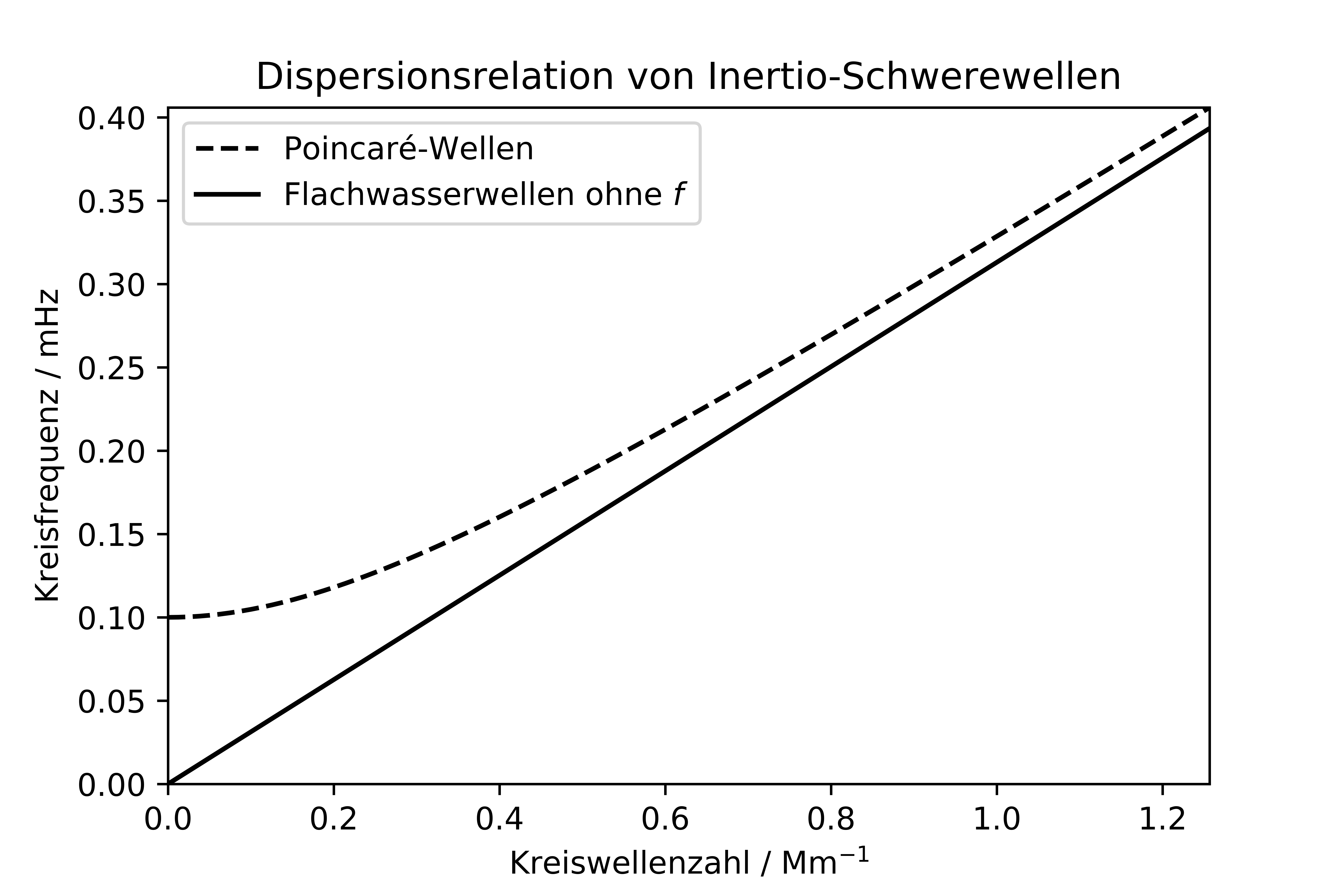
\[ \begin{align} c^2 = \frac{\omega^2}{k^2} = gH + \frac{f^2}{k^2} = gH + f^2L^2\frac{1}{4\pi^2} \end{align} \]

with $L$ denoting the wavelength. Poincaré waves therefore have a higher phase speed than gravity waves without Earth's rotation. The shorter the waves, the weaker the influence of the Coriolis force; for long waves, however, $\omega$ approaches $f$. Relative to gravity waves without Coriolis force, the expression for $c^2$ is larger by $f^2L^2\frac{1}{4\pi^2}$. To determine a cutoff wavelength $R_o$ from which the Coriolis effect becomes significant, one sets

\[ \begin{align} f_0^2R_o^2\frac{1}{4\pi^2} = \frac{gH}{4\pi^2}\approx 0, 025gH. \end{align} \]

This gives the barotropic Rossby radius

\[ \begin{align} R_o = \frac{\sqrt{gH}}{\left|f\right|}.\tag{16.107}\label{eq:def_baro_ro_r} \end{align} \]

Using typical values, one obtains $R_o \approx 2000$ km.

Poincaré waves are also known as inertia-gravity waves, since their restoring forces are gravity and the Coriolis force. Another name is Sverdrup wave.

16.5.4 Kelvin waves

One starts again from the system of equations (16.89) - (16.91), but this time one imagines the half-plane $x<0$ as a coast, so that only the remaining half-plane $x\geq 0$ can be flowed through by the fluid. The boundary condition is therefore:

\[ \begin{align} u\left(x = 0\right) = 0. \end{align} \]

One now seeks solutions that satisfy this globally. To this end, one again starts from the f-plane. The system of equations reduces to

\[ \begin{align} 0 &= -g\frac{\partial\eta}{\partial x} + fv, \tag{16.109}\label{eq:kelvin_1}\\ \frac{\partial v}{\partial t} &= -g\frac{\partial\eta}{\partial y}, \tag{16.110}\label{eq:kelvin_2}\\ \frac{\partial\eta}{\partial t} + H \frac{\partial v}{\partial y} &= 0.\tag{16.111}\label{eq:kelvin_3} \end{align} \]

From Eq. (16.109) it follows that $v$ is geostrophically balanced, so one can eliminate $v$ from the remaining two equations:

\[ \begin{align} \frac{\partial^2\eta}{\partial t\partial x} &= -f\frac{\partial\eta}{\partial y},\\ \frac{\partial\eta}{\partial t} + H\frac{g}{f}\frac{\partial^2\eta}{\partial x\partial y} &= 0. \end{align} \]

Here one makes the harmonic wave ansatz

\[ \begin{align} \eta = \eta_0\exp\left[i\left(k_xx + k_yy - \omega t\right)\right], \end{align} \]

from which it follows that

\[ \begin{align} -iwik_x &= -fik_y\Rightarrow wk_x = -ifk_y, \tag{16.115}\label{eq:kelvin_deriv_1}\\ -i\omega + H\frac{g}{f}ik_xik_y &= 0 \Rightarrow i\omega = -H\frac{g}{f}k_xk_y.\tag{16.116}\label{eq:kelvin_deriv_2} \end{align} \]

From Eq. (16.115) follows

\[ \begin{align} k_x = -\frac{i}{\omega}fk_y, \end{align} \]

which, substituted into Eq. (16.116),

\[ \begin{align} i\omega &= -H\frac{g}{f}k_y\left(-\frac{i}{\omega}fk_y\right) = iH\frac{g}{\omega}k_y^2 \end{align} \]

yields. Defining $\kappa$ by

\[ \begin{align} \kappa \coloneqq \frac{\omega}{\sqrt{gH}} > 0 \end{align} \]

with an angular frequency $\omega > 0$ assumed to be positive, one obtains

\[ \begin{align} k_y = \pm\kappa.\tag{16.120}\label{eq:kelvin_deriv_3} \end{align} \]

Rearranged, this yields

With Eq. (16.115), it follows that

$\eta$ must not grow exponentially as a function of the distance from the coast; therefore, for $f > 0$ the negative sign in Eq. (16.120) holds, and for $f < 0$ the positive one. In the northern hemisphere the Kelvin wave thus has the coast to the right of the direction of propagation, in the southern hemisphere to the left.

The penetration lengths $l$ of the Kelvin waves are:

with the Rossby radius $R_o$ defined in Eq. (16.107).

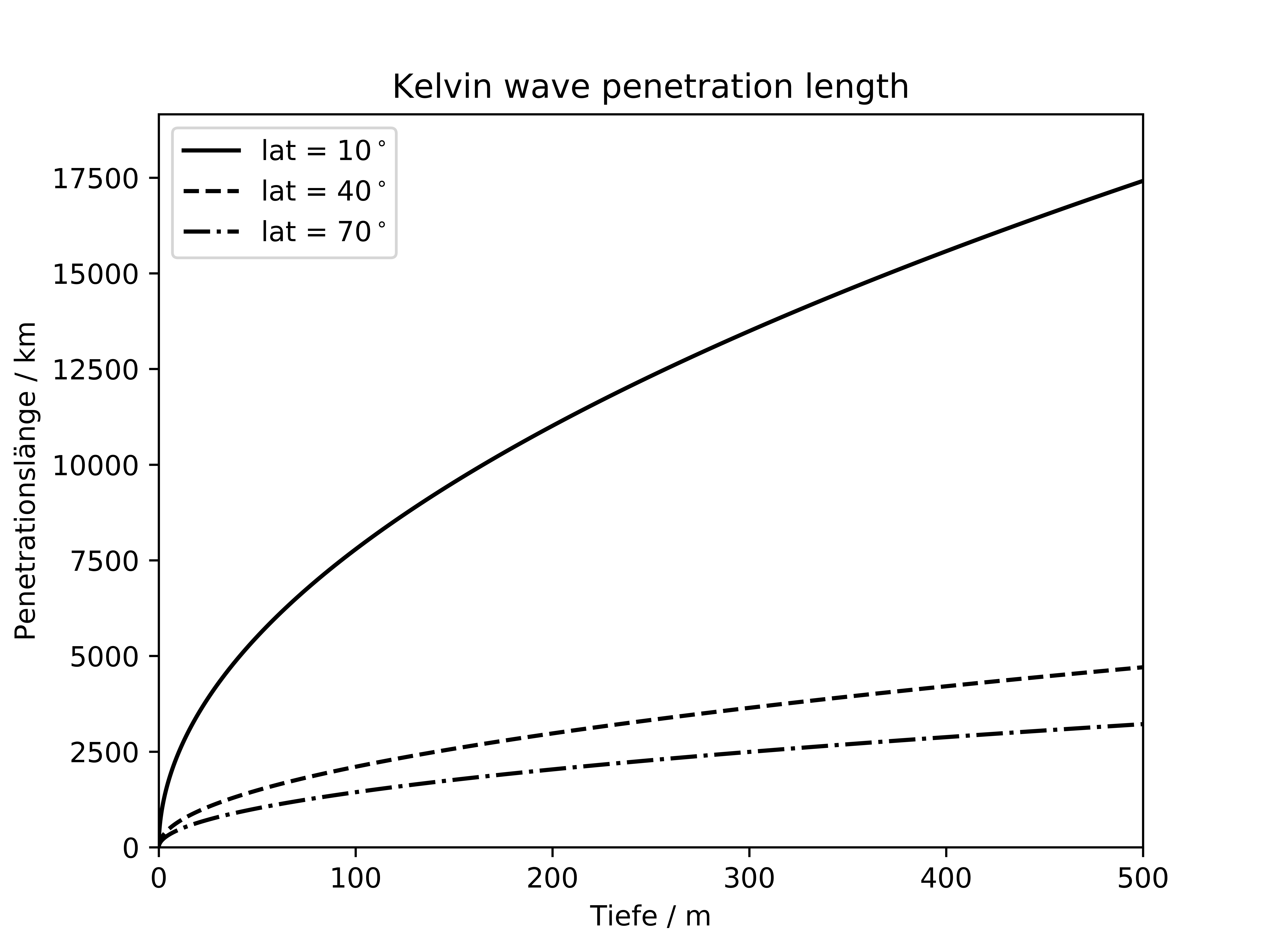
Fig. 16.2 shows the typical penetration lengths of Kelvin waves, which quickly lie in the range of $1000$ - $10000$ km, i.e. in the range of ten to several hundred percent of a quarter of the Earth's circumference. This extent far exceeds the range of validity of the f-plane.

16.5.4.1 Equatorial Kelvin waves

At the equator, one cannot set $f = f_0$; instead one adopts the $\beta$-plane

\[ \begin{align} f = \beta y \end{align} \]

with

\[ \begin{align} \beta \coloneqq \frac{\partial f}{\partial y}\newvline_{\varphi = 0}. \end{align} \]

With this, Eqs. (16.89) - (16.91) read

\[ \begin{align} \frac{\partial u}{\partial t} &= -g\frac{\partial\eta}{\partial x} + \beta yv,\\ \frac{\partial v}{\partial t} &= -g\frac{\partial\eta}{\partial y} - \beta yu,\\ \frac{\partial\eta}{\partial t} + H\left(\frac{\partial u}{\partial x} + \frac{\partial v}{\partial y}\right) &= 0. \end{align} \]

One now seeks solutions with $v = 0$. In this case, one has

\[ \begin{align} \frac{\partial u}{\partial t} &= -g\frac{\partial\eta}{\partial x},\\ 0 &= -g\frac{\partial\eta}{\partial y} - \beta yu,\\ \frac{\partial\eta}{\partial t} + H\frac{\partial u}{\partial x} &= 0. \end{align} \]

Over

\[ \begin{align} u = -\frac{g}{\beta y}\frac{\partial\eta}{\partial y} \end{align} \]

$u$ can be eliminated:

\[ \begin{align} -\frac{g}{\beta y}\frac{\partial^2\eta}{\partial t\partial y} &= -g\frac{\partial\eta}{\partial x}\\ \frac{\partial\eta}{\partial t} - \frac{gH}{\beta y}\frac{\partial^2\eta}{\partial x\partial y} &= 0 \end{align} \]

The ansatz

\[ \begin{align} \eta = \newhat{\eta}\exp\left[i\left(k_xx + k_yy -\omega t\right)\right] \end{align} \]

leads to

\[ \begin{align} -\frac{g}{\beta y}k_y\omega &= -gik_x \Rightarrow k_y = \frac{1}{\omega}\beta yik_x,\\ -i\omega + \frac{gH}{\beta y}k_xk_y &= 0 \Rightarrow \omega^2 = gHk_x^2. \end{align} \]

One thus has

\[ \begin{align} k_x = \pm\frac{\omega}{\sqrt{gH}}. \end{align} \]

For $k_y$, it follows that

\[ \begin{align} k_y = \frac{1}{\omega}\beta yik_x = \pm i\frac{\beta y}{\sqrt{gH}}. \end{align} \]

Only the plus sign is admissible. The solution is therefore

To estimate the meridional extent $y_0$ of these waves, one sets

\[ \begin{align} 1 = \frac{2\omega y_0^2}{\sqrt{gH}} \end{align} \]

From this it follows

\[ \begin{align} y_0 =\sqrt{R\frac{\sqrt{gH}}{2\omega}} = 2071\text{ km} \end{align} \]

with $R$ the equatorial radius and $H = 1$ km.

16.5.5 Rossby-Haurwitz modes

Rossby-Haurwitz modes are the eigenmodes of the barotropic vorticity equation Eq. (15.92) on the sphere. Therefore, the notation from Sect. 15.1.3.6 is adopted in this section. Spherical surface functions $Y_{l, m}\left(\phi, \lambda\right)$ with $l \geq 0$ and $-l \leq m \leq l$ satisfy

\[ \begin{align} \Delta Y_{l, m} \stackrel{\href{ch-41-orthogonal-function-systems.html#eq:spherical_harm_prop_1}{\text{Eq. (C.166)}}}{=} -\frac{l\left(l + 1\right)}{a^2}Y_{l, m}. \end{align} \]

Making, for the stream function $\psi = \psi\left(\phi, \lambda, t\right)$, the ansatz

\[ \begin{align} \psi = Y_{l, m}e^{-i\omega t},\tag{16.144}\label{eq:rossby-haurwitz_ansatz} \end{align} \]

it follows that

\[ \begin{align} J\left(\zeta, \psi\right) = J\left(\Delta\psi, \psi\right) \propto \frac{\partial\psi}{\partial\lambda}\frac{\partial\psi}{\partial\phi} - \frac{\partial\psi}{\partial\phi}\frac{\partial\psi}{\partial\lambda} = 0. \end{align} \]

Substituting Eq. (16.144) into the barotropic vorticity equation in the form Eq. (15.101), one thus obtains

\[ \begin{align} \Delta\frac{\partial\psi}{\partial t} &= -\frac{\partial\psi}{a\cos\left(\phi\right)\partial\lambda}\beta + \frac{1}{a^2\cos\left(\phi\right)}J\left(\Delta\psi, \psi\right) = -\frac{\partial\psi}{a\cos\left(\phi\right)\partial\lambda}\beta\nonumber\\ \Delta\frac{\partial\psi}{\partial t} &= -\frac{\partial\psi}{a^2\cos\left(\phi\right)\partial\lambda}2\omega\cos\left(\phi\right) = -\frac{\partial\psi}{a^2\partial\lambda}2\Omega\nonumber\\ \Rightarrow-i\omega l\frac{l\left(l + 1\right)}{a^2} &= -\frac{2\Omega}{a^2}im\nonumber\\ \Rightarrow\omega\frac{l\left(l + 1\right)}{a^2} &= \frac{2\Omega}{a^2}m\tag{16.146}\label{eq:rossby-haurwitz_disprel_deriv} \end{align} \]

From this, the dispersion relation of the Rossby-Haurwitz modes follows:

In the case $l = 0$, one has $m = 0$, and Eq. (16.146) is satisfied for every $\omega$. From Eq. (16.147), it follows that

\[ \begin{align} -\frac{1}{\left(l + 1\right)}2\Omega \leq \omega\left(l, m\right) \leq \frac{1}{\left(l + 1\right)}2\Omega. \end{align} \]

For the phase velocity (expressed as zonal angular velocity) one obtains

\[ \begin{align} \frac{\omega}{\frac{2\pi}{\Delta\lambda}} = \frac{\omega\Delta\lambda}{2\pi} = \frac{\omega 2\pi}{2\pi m} = \frac{\omega}{m} = \frac{1}{l\left(l + 1\right)}2\Omega > 0. \end{align} \]

Rossby-Haurwitz modes therefore always propagate eastward. By means of Eq. (15.139), which reads

\[ \begin{align} \Delta\Phi = \beta\frac{\partial\psi}{\partial y} + f\Delta\psi, \end{align} \]

The geopotential $\Phi$ can be determined from $\psi$. First one inserts a Rossby-Haurwitz mode

\[ \begin{align} \psi = \psi_0Y_{l, m}e^{-i\omega t} \end{align} \]

, this implies

\[ \begin{align} \Delta\Phi &= \frac{2\Omega\cos\left(\phi\right)}{a^2\cos\left(\phi\right)}\frac{\partial\psi}{\partial\phi} - \frac{2\Omega\sin\left(\phi\right)}{a^2}l\left(l + 1\right)\psi_0Y_{l, m}e^{-i\omega t}\nonumber\\ \Rightarrow\Delta\Phi &= \frac{2\Omega}{a^2}\frac{\partial\psi}{\partial\phi} - \frac{2\Omega\sin\left(\phi\right)}{a^2}l\left(l + 1\right)\psi_0Y_{l, m}e^{-i\omega t}. \end{align} \]

For the geopotential $\Phi$, one now makes the ansatz

\[ \begin{align} \Phi = \sum_{l' = 0}^\infty\sum_{m' = -l'}^{l'}\Phi_{l', m'}Y_{l', m'}. \end{align} \]

Substituting this, one obtains

\[ \begin{align} \sum_{l' = 0}^\infty\sum_{m' = -l'}^{l'}-\frac{l'\left(l' + 1\right)}{a^2}\Phi_{l', m'}Y_{l', m'} &= \frac{2\Omega}{a^2}\frac{\partial\psi}{\partial\phi} - \frac{2\Omega\sin\left(\phi\right)}{a^2}l\left(l + 1\right)\psi_0Y_{l, m}e^{-i\omega t}\nonumber\\ \Rightarrow\sum_{l' = 0}^\infty\sum_{m' = -l'}^{l'}-l'\left(l' + 1\right)\Phi_{l', m'}Y_{l', m'} &= 2\Omega\frac{\partial\psi}{\partial\phi} - 2\Omega\sin\left(\phi\right)l\left(l + 1\right)\psi_0Y_{l, m}e^{-i\omega t}. \end{align} \]

Eq. (C.180) reads

\[ \begin{align} \sin\left(\phi\right)Y_{l, m} = \sqrt{\frac{l^2 - m^2}{4l^2 - 1}}Y_{l - 1, m} + \sqrt{\frac{\left(l + 1\right)^2 - m^2}{4\left(l + 1\right)^2 - 1}}Y_{l + 1, m}. \end{align} \]

This implies

\[ \begin{align} \sum_{l' = 0}^\infty\sum_{m' = -l'}^{l'}-l'\left(l' + 1\right)\Phi_{l', m'}Y_{l', m'} &= 2\Omega\frac{\partial\psi}{\partial\phi} - 2\Omega l\left(l + 1\right)\psi_0\left[\sqrt{\frac{l^2 - m^2}{4l^2 - 1}}Y_{l - 1, m} + \sqrt{\frac{\left(l + 1\right)^2 - m^2}{4\left(l + 1\right)^2 - 1}}Y_{l + 1, m}\right]e^{-i\omega t}. \end{align} \]

16.5.6 Barotropic Rossby waves

In Sect. 16.5.3 $\beta = 0$ was assumed. In this case, the Poincaré waves derived there are the most general wave solutions. A new type of waves arises when the width dependence of $f$ is taken into account.

One starts from a homogeneous zonal base current $U$. One assumes $u_0 = 0$ and also $k_y = 0$; the perturbations should depend only on x. One already knows:

• Since $U$ is homogeneous and $u_0 = 0$, $v = v\left(x, t\right)$ hold, the solutions are divergence-free.

Therefore one can use the barotropic vorticity equation. Making the ansatz

\[ \begin{align} v = v_0\exp\left[i\left(kx - \omega t\right)\right] \end{align} \]

the following hold

\[ \begin{align} \zeta = ikv, & {} & \frac{\partial\zeta}{\partial t} = k\omega v, & {} & \frac{\partial\zeta}{\partial x} = -k^2v. \end{align} \]

Substituting this into the barotropic vorticity equation, one obtains

\[ \begin{align} k\omega v_0 &= Uk^2v_0 - v_0\beta\Leftrightarrow\omega = Uk - \frac{\beta}{k}.\tag{16.159}\label{eq:rossby_welle_barotrop_disp} \end{align} \]

Eq. (16.159) is the dispersion relation of barotropic Rossby waves. If they span a complete circle of latitude, they are also referred to as planetary waves.

The following applies to the phase velocity of barotropic Rossby waves

In the hypothetical case $U\to0$, $L = 2\pi a$ and $\varphi = 0$, one has

\[ \begin{align} \left|c\right| = 2\omega\frac{1}{a}\frac{4\pi^2 a^2}{4\pi^2} = 2\omega a = 930\:\frac{\text{m}}{\text{s}}. \end{align} \]

This is a bound on the magnitude of $c$. No wave can propagate faster than the speed $2\omega a$, and the system of governing equations cannot transmit information any faster.

16.5.6.1 Intuitive understanding

The y-component of the momentum equation in the shallow-water model reads

\[ \begin{align} \md{v} = -fu - g\frac{\partial\eta}{\partial y}.\tag{16.162}\label{eq:momentum_swe_y} \end{align} \]

One performs a linear Taylor expansion for $f$

\[ \begin{align} f = f_0 + \beta y. \end{align} \]

A homogeneous zonal base current $U$ can be geostrophically balanced by a surface deflection

\[ \begin{align} 0 = -f_0U - g\frac{\partial\eta}{\partial y}. \end{align} \]

In this case, Eq. (16.162) becomes

\[ \begin{align} \md{^2y}{t^2} = -\beta U y. \end{align} \]

This corresponds to a harmonic oscillator with the natural frequency

\[ \begin{align} \omega_{\text{ind}} = \sqrt{\beta U}. \end{align} \]

Therefore $U>0$ must be westerly. The natural frequency was marked with an index $\text{ind}$ because it is the individual oscillation frequency of the particles and not the frequency $\omega$ of the wave.

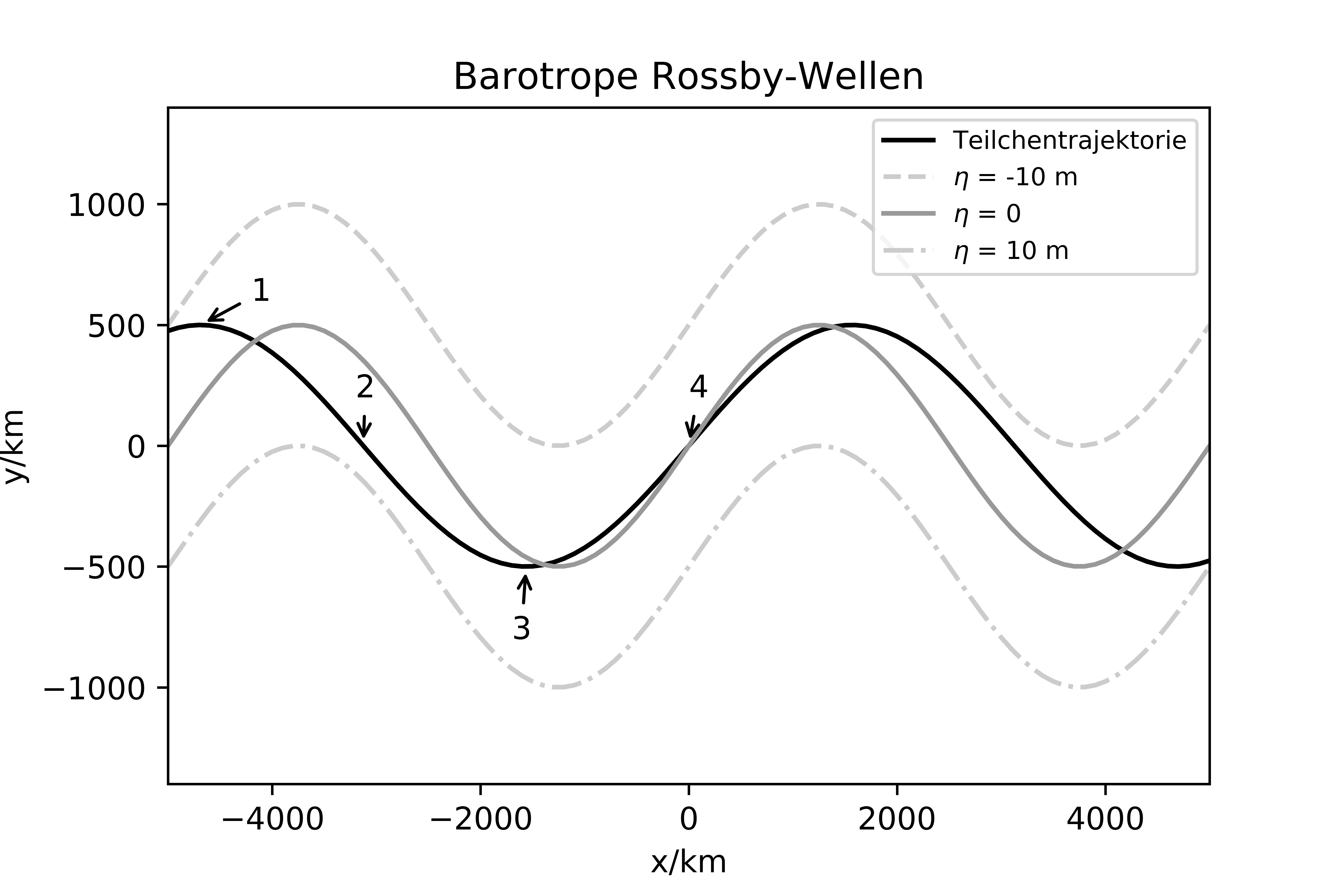
Another intuitive explanation follows from the barotropic vorticity equation, which reads:

\[ \begin{align} f + \zeta = \text{const}. \end{align} \]

If a particle is deflected northward from its rest position in the northern hemisphere in the presence of a westerly base current, then $f$ increases. Therefore $\zeta$ must decrease and the particle acquires anticyclonic relative vorticity. It then oscillates southward beyond its rest position, with $f$ decreasing. Therefore, the particle acquires cyclonic relative vorticity and veers northward again. The mechanism of barotropic Rossby waves is the conservation of absolute vorticity, see also Fig. 16.3.

Barotropic Rossby waves are relevant in the atmosphere and ocean despite the extensive simplifications (barotropy and non-divergence). In the atmosphere, due to their non-divergence, they are most applicable to the middle troposphere and provide a simple view of the meandering polar jet. The term wave number is often used here; a wave of wave number $n$ has a zonal spatial period of $\frac{2\pi}{n}$ as an angle. Rossby waves always propagate westward in the ocean due to the small easterly (eastward-directed) base current (it is $\beta\geq0$ over the entire Earth).

16.5.7 Oceanic tide

The oceanic tide is a global phenomenon, so advection ($\propto 1/\lambda$) can be neglected. Barotropy can also be assumed. Therefore, the linear shallow-water equations Eqs. (13.173) - (13.174) are used as the system of equations. In components, these read

\[ \begin{align} \frac{\partial u}{\partial t} &= -\frac{\partial\left(gd + U\right)}{a\cos\left(\phi\right)\partial\lambda} + 2\Omega\sin\left(\phi\right)v,\\ \frac{\partial v}{\partial t} &= -\frac{\partial\left(gd + U\right)}{a\partial\phi} - 2\Omega\sin\left(\phi\right)u,\\ \frac{\partial d}{\partial t} &= -D\left(\frac{\partial u}{a\cos\left(\phi\right)\partial\lambda} + \frac{\partial v}{a\partial\phi} - v\frac{\tan\left(\phi\right)}{a}\right). \end{align} \]

Here $U = U\left(\phi, \lambda, t\right)$ is the tidal potential. $\Omega$ is the angular velocity of the Earth's rotation. These equations are also known as Laplace's tidal equations (LTEs). Here one makes the ansatz

\[ \begin{align} u = \sum_{l = 0}^\infty\sum_{m = -l}^l\newtilde{u}_{l, m}Y_{l, m}\left(\phi, \lambda\right)e^{-i\omega t}, & {} & v = \sum_{l = 0}^\infty\sum_{m = -l}^l\newtilde{v}_{l, m}Y_{l, m}\left(\phi, \lambda\right)e^{-i\omega t},\\ d = \sum_{l = 0}^\infty\sum_{m = -l}^l\newtilde{d}_{l, m}Y_{l, m}\left(\phi, \lambda\right)e^{-i\omega t}, & {} & U = \sum_{l = 0}^\infty\sum_{m = -l}^l\newtilde{U}_{l, m}Y_{l, m}\left(\phi, \lambda\right)e^{-i\omega t}, \end{align} \]

Here $Y_{l, m}\left(\phi, \lambda\right)$ are spherical surface functions, see Sect. C.5. The following hold:

\[ \begin{align} \frac{\partial Y_{l, m}}{\partial\phi} &\stackrel{\href{ch-41-orthogonal-function-systems.html#eq:spherical_harmonic_deriv_theta}{\text{Eq. (C.167)}}}{=} -m\tan\left(\phi\right) Y_{l, m} - \sqrt{l^2 - m^2 + l - m}Y_{l, m + 1}\exp\left(-i\lambda\right),\\ \frac{\partial Y_{l, m}}{\partial\lambda} &\stackrel{\href{ch-41-orthogonal-function-systems.html#eq:spherical_harmonic_deriv_phi}{\text{Eq. (C.168)}}}{=} imY_{l, m},\\ \sin\left(\phi\right)Y_{l, m} &\stackrel{\href{ch-41-orthogonal-function-systems.html#eq:spherical_harm_prop_2}{\text{Eq. (C.171)}}}{=} \sqrt{\frac{l^2 - m^2}{4l^2 - 1}}Y_{l - 1, m} + \sqrt{\frac{\left(l + 1\right)^2 - m^2}{4\left(l + 1\right)^2 - 1}}Y_{l + 1, m}. \end{align} \]

With the abbreviations

\[ \begin{align} f_{l, m} = \sqrt{l^2 - m^2 + l - m},& {} & g_{l, m} = \sqrt{\frac{l^2 - m^2}{4l^2 - 1}},& {} & h_{l, m} = \sqrt{\frac{\left(l + 1\right)^2 - m^2}{4\left(l + 1\right)^2 - 1}} \end{align} \]

one can write this in the form

\[ \begin{align} \frac{\partial Y_{l, m}}{\partial\phi} &\stackrel{\href{ch-41-orthogonal-function-systems.html#eq:spherical_harmonic_deriv_theta_geo}{\text{Eq. (C.178)}}}{=} -m\tan\left(\phi\right) Y_{l, m} - f_{l, m}Y_{l, m + 1}\exp\left(-i\lambda\right),\\ \frac{\partial Y_{l, m}}{\partial\lambda} &\stackrel{\href{ch-41-orthogonal-function-systems.html#eq:spherical_harmonic_deriv_phi_geo}{\text{Eq. (C.179)}}}{=} imY_{l, m},\\ \sin\left(\phi\right)Y_{l, m} &\stackrel{\href{ch-41-orthogonal-function-systems.html#eq:spherical_harm_prop_2_geo}{\text{Eq. (C.180)}}}{=} g_{l, m}Y_{l - 1, m} + h_{l, m}Y_{l + 1, m} \end{align} \]

Substituting all of this into the LTEs, one obtains

\[ \begin{align} &-i\omega\sum_{l = 0}^\infty\sum_{m = -l}^l\newtilde{u}_{l, m}Y_{l, m}\nonumber\\ &= \sum_{l = 0}^\infty\sum_{m = -l}^l-im\frac{g\newtilde{d}_{l, m} + \newtilde{U}_{l, m}}{a\cos\left(\phi\right)}Y_{l, m} + 2\Omega\newtilde{v}_{l, m}\left(g_{l, m}Y_{l - 1, m} + h_{l, m}Y_{l + 1, m}\right),\\ &-i\omega\sum_{l = 0}^\infty\sum_{m = -l}^l\newtilde{v}_{l, m}Y_{l, m}\nonumber\\ &= \sum_{l = 0}^\infty\sum_{m = -l}^l\frac{g\newtilde{d}_{l, m} + \newtilde{U}_{l, m}}{a}\left(m\tan\left(\phi\right) Y_{l, m} + f_{l, m}Y_{l, m + 1}\exp\left(-i\lambda\right)\right) - 2\Omega\newtilde{u}_{l, m}\left(g_{l, m}Y_{l - 1, m} + h_{l, m}Y_{l + 1, m}\right),\\ &-i\omega\sum_{l = 0}^\infty\sum_{m = -l}^l\newtilde{d}_{l, m}Y_{l, m}\nonumber\\ &= -\frac{D}{a}\sum_{l = 0}^\infty\sum_{m = -l}^lim\frac{\newtilde{u}_{l, m}}{\cos\left(\phi\right)}Y_{l, m} - \newtilde{v}_{l, m}\left(m\tan\left(\phi\right) Y_{l, m} + f_{l, m}Y_{l, m + 1}\exp\left(-i\lambda\right)\right) - \newtilde{v}_{l, m}\tan\left(\phi\right)Y_{l, m}\nonumber\\ &= -\frac{D}{a}\sum_{l = 0}^\infty\sum_{m = -l}^lim\frac{\newtilde{u}_{l, m}}{\cos\left(\phi\right)}Y_{l, m} - \newtilde{v}_{l, m}\left[\left(m + 1\right)\tan\left(\phi\right) Y_{l, m} + f_{l, m}Y_{l, m + 1}\exp\left(-i\lambda\right)\right]. \end{align} \]

Coastlines, bathymetry, and bottom friction modify this significantly.

16.5.7.1 Intuitive understanding

In contrast to many illustrative figures, it is not so much the vertical but predominantly the horizontal component of $-\nabla U$ that is relevant for the oceanic tide. However, what is somewhat counterintuitive is the fact that in most places it is not the period $\sim$ 25 hours that predominates, but rather the first harmonic of the lunar tide with a period of $\sim$ 12.5 hours. To understand this intuitively, one places a coordinate system at the center of the Earth and aligns the negative x-axis with the Moon. Lunar quantities (referring to the Moon) are denoted by the index $l$ and terrestrial quantities by the index $t$. For the x-coordinate $x_S$ of the center of gravity one obtains

\[ \begin{align} x_S = \frac{m_lx_l + m_tx_t}{m_l + m_t} = \frac{m_lx_l}{m_l + m_t} = \frac{1}{1 + \frac{m_t}{m_l}}x_l = -0,73 a. \end{align} \]

The center of gravity of the Moon and Earth therefore lies within the Earth. At the point $x = -a$, the tidal force $\mathbf{f}_T$ is thus directed towards the Moon. At $x = a$, one has

\[ \begin{align} f_{T, x} = \omega_l^2\left(a - x_S\right) - \frac{Gm_l}{\left(a - x_l\right)^2} = 1,73\omega_l^2a - \frac{Gm_l}{\left(a - x_l\right)^2}. \end{align} \]

$\omega_l$ is the angular velocity of the Moon's rotation around the Earth. It is easy to verify that

\[ \begin{align} f_{T, x} > 0 \end{align} \]

holds. At the two points considered so far, the tidal force has no horizontal component. If one moves away from these points, the horizontal tidal force is directed towards these points. This implies that there must be another point on every semicircle between $x = -a$ and $x = a$ where $\mathbf{f}_T = -\nabla U$ has no horizontal component. This suggests that the period $\sim$ 12.5 hours is more dominant than the lunar fundamental period.

16.6 Baroclinic waves

16.6.1 Vertical modes

Here one assumes a flat bottom at a depth $z = -D < 0$ and imposes the boundary conditions

\[ \begin{align} w\left(z = 0\right) &= 0,\\ w\left(z = -D\right) &= 0. \end{align} \]

One uses the following system of equations, assuming without loss of generality a wave propagating in the x direction:

\[ \begin{align} \frac{\partial u}{\partial t} &= -\frac{1}{\rho_0}\frac{\partial p'}{\partial x},\\ \frac{\partial w}{\partial t} &= -\frac{1}{\rho_0}\frac{\partial p'}{\partial z},\\ \frac{\partial\rho'}{\partial t} &= -\rho_0\frac{\partial u}{\partial x} - \rho_0\frac{\partial w}{\partial z}. \end{align} \]

Here

\[ \begin{align} \rho = \rho_0 + \rho' \end{align} \]

with a homogeneous background density $\rho_0$ and a fluctuation $\rho'$. Analogously, one decomposes the pressure $p$, where the following should hold:

\[ \begin{align} \frac{\partial p_0}{\partial z} = -g\rho_0. \end{align} \]

One now makes the ansätze

\[ \begin{align} u = U\left(z\right)\exp\left(ikx-i\omega t\right), & {} & v = V\left(z\right)\exp\left(ikx-i\omega t\right),\\ p' = P\left(z\right)\exp\left(ikx-i\omega t\right), & {} & \rho' = \newtilde{\rho}\left(z\right)\exp\left(ikx-i\omega t\right). \end{align} \]

Substituting this into the governing system of equations, it follows

\[ \begin{align} -i\omega U = -\frac{ikP}{\rho_0} \Rightarrow \omega U &= \frac{kP}{\rho_0}, \tag{16.195}\label{eq:v_mode_deriv_2}\\ -i\omega W = -\frac{P'}{\rho_0} \Rightarrow \omega W &= -i\frac{P'}{\rho_0}, \tag{16.196}\label{eq:v_mode_deriv_1}\\ -i\omega\newtilde{\rho} = -\rho_0ikU - \rho_0W' \Rightarrow \omega\newtilde{\rho} &= \rho_0kU - i\rho_0W'. \end{align} \]

The third equation is always satisfiable, $\newtilde{\rho}\left(z\right)$ can be chosen accordingly. For $W$, one makes the ansatz

\[ \begin{align} W\left(z\right) = \newhat{w}\sin\left(n\pi\frac{z}{D}\right) \end{align} \]

with $n\geq 1$. From Eq. (16.196), it follows that

\[ \begin{align} P' = \rho_0i \omega\newhat{w}\sin\left(n\pi\frac{z}{D}\right). \end{align} \]

For $P$, one therefore sets

\[ \begin{align} P\left(z\right) = -\frac{D\rho_0i\omega\newhat{w}}{n\pi}\cos\left(n\pi\frac{z}{D}\right) \end{align} \]

Substituting this into Eq. (16.196), it follows that

\[ \begin{align} U\left(z\right) = \frac{kP}{\omega\rho_0} = -\frac{ki\newhat{w}D}{n\pi}\cos\left(n\pi\frac{z}{D}\right). \end{align} \]

One thus has

\[ \begin{align} u\left(x, z, t\right) &= \frac{Dk\newhat{w}}{n\pi}\cos\left(n\pi\frac{z}{D}\right)\exp\left[i\left(kx - \omega t - \frac{\pi}{2}\right)\right]\nonumber\\ \Rightarrow u\left(x, z, t\right) &= -i\frac{Dk\newhat{w}}{n\pi}\cos\left(n\pi\frac{z}{D}\right)\exp\left[i\left(kx - \omega t\right)\right]\nonumber\\ \Rightarrow u\left(x, z, t\right) &= -i\frac{Dk\newhat{w}}{n\pi}\cos\left(n\pi\frac{z}{D}\right)\left[\cos\left(kx - \omega t\right) + i\sin\left(kx - \omega t\right)\right]\nonumber\\ \Rightarrow u\left(x, z, t\right) &= \frac{Dk\newhat{w}}{n\pi}\cos\left(n\pi\frac{z}{D}\right)\left[-i\cos\left(kx - \omega t\right) + \sin\left(kx - \omega t\right)\right]\nonumber\\ \Rightarrow\Re\left(u\left(x, z, t\right)\right) &= \frac{Dk\newhat{w}}{n\pi}\cos\left(n\pi\frac{z}{D}\right)\sin\left(kx - \omega t\right). \end{align} \]

The horizontal divergence $\delta$ at the surface is given by

\[ \begin{align} \delta\left(z = 0\right) = \frac{\partial\Re\left(u\left(x, z, t\right)\right)}{\partial x} = \frac{Dk^2\newhat{w}}{n\pi}\cos\left(n\pi\frac{z}{D}\right)\cos\left(kx - \omega t\right). \end{align} \]

Vertical modes therefore lead to alternating stripes of divergence and convergence at the surface. In the area of convergence, the surface waves are compressed horizontally, which destabilizes the wave field. Conversely, the wave field is stabilized in the area of ​​divergence, which also contributes to the fact that in this region water rises from the depths to the surface, water that has not yet been exposed to the action of the wind.

The mode $n = 0$ is also called the external mode, since it has no internal vertical structure.

16.6.2 Gravity waves

Baroclinic gravity waves are the baroclinic analogue of Poincaré waves. First one makes a perturbation ansatz of the form

\[ \begin{align} u = U + u', & {} & v = v', & {} & w = w',\tag{16.204}\label{eq:gw_disp_deriv_0}\\ p = p_0\left(z\right) + p', & {} & \theta = \theta_0\left(z\right) + \theta', & {} & f = f_0.\tag{16.205}\label{eq:gw_disp_deriv_1} \end{align} \]

Because of Eq. (16.205), Eq. (16.204) is not a restriction of the background current to the x-direction; by rotating the coordinate system around the vertical axis, the background wind can assume any direction. In particular, all curvature terms are neglected and one can use Cartesian coordinates $\left(x, y, z\right)$. The background state is required to be hydrostatic, i.e. to satisfy

\[ \begin{align} \frac{\partial p_0}{\partial z} = -g\rho_0\left(z\right)\tag{16.206}\label{eq:hydrostatic_gravity_wave} \end{align} \]

A dry adiabatic system is assumed; in such a system the first law of thermodynamics becomes

\[ \begin{align} \md{\theta} = 0 & {} & \Leftrightarrow & {} & \md{\theta} + \md{\theta'} = 0 & {} & \Leftrightarrow \md{\theta'} + w'\frac{d\theta_0}{dz} = 0. \end{align} \]

One now introduces an approximate material derivative $\mdtilde{}$ in which perturbation products are neglected. In the following, equals signs are written for it. One thus obtains

\[ \begin{align} \mdtilde{\theta'} + w'\frac{d\theta_0}{dz} &= 0. \end{align} \]

If one multiplies this equation by $\frac{g}{\theta_0}$, it follows

\[ \begin{align} \mdtilde{b'} + w'\frac{g}{\theta_0}\frac{d\theta_0}{dz} = 0, \end{align} \]

where the definition of the so-called buoyancy

\[ \begin{align} b' \coloneqq g\frac{\theta'}{\theta_0} \end{align} \]

was used. From Eq. (16.253), one reads off

\[ \begin{align} \frac{g}{\theta_0}\frac{d\theta_0}{dz} = N^2, \end{align} \]

which leads to

\[ \begin{align} \mdtilde{b'} + w'N^2 = 0. \end{align} \]

With Eq. (9.69), one obtains

\[ \begin{align} \md{p} + \frac{c^{(p)}}{c^{(V)}}p\nabla\cdot\mathbf{v} &= 0\nonumber\\ \Leftrightarrow \frac{1}{\kappa p}\md{p} + \nabla\cdot\mathbf{v} &= 0\nonumber\\ \Leftrightarrow \frac{1}{\kappa\rho R_dT}\md{p} + \nabla\cdot\mathbf{v} &= 0. \end{align} \]

With Eq. (16.42) this can be expressed in terms of the speed of sound:

\[ \begin{align} \frac{1}{c_s^2\rho}\md{p} + \nabla\cdot\mathbf{v} &= 0 \end{align} \]

Linearizing this equation, one obtains

\[ \begin{align} \frac{1}{c_s^2\rho}\mdtilde{p} + \nabla\cdot\mathbf{v}' &= 0\nonumber\\ \Leftrightarrow \frac{1}{c_s^2\rho_0}\mdtilde{p}' + \frac{1}{c_s^2\rho_0}w'\frac{dp_0}{dz} + \nabla\cdot\mathbf{v}' &= 0\nonumber\\ \Leftrightarrow \frac{1}{c_s^2\rho_0}\mdtilde{p}' - \frac{g}{c_s^2}w' + \nabla\cdot\mathbf{v}' &= 0. \end{align} \]

For the vertical equation of motion, one obtains using Eq. (13.151)

\[ \begin{align} \mdtilde{w'} = -g - \frac{1}{\rho}\frac{\partial p}{\partial z} = -\frac{1}{\rho}\frac{\partial p'}{\partial z} - \left(\frac{1}{\rho}\right)'\frac{\partial p_0}{\partial z} \approx - \frac{1}{\rho_0}\frac{\partial p'}{\partial z} + \frac{\rho'}{\rho_0^2}\frac{\partial p_0}{\partial z} = -\frac{1}{\rho_0}\frac{\partial p'}{\partial z} - \frac{g\rho'}{\rho_0}. \end{align} \]

To express the perturbation in the density through perturbations in the potential temperature and pressure, one writes Eq. (9.65) in the form

\[ \begin{align} \rho = \frac{p_\text{ref}^{R_d/c^{(p)}}}{R_d}\frac{p^{1/\kappa}}{\theta}. \end{align} \]

To first order, one thus has

\[ \begin{align} \rho' &= \frac{1}{\kappa}\frac{\rho_0}{p_0}p' - \frac{\rho_0}{\theta}\theta' \approx \frac{p'}{c_s^2} - \frac{\rho_0}{\theta_0}\theta' \end{align} \]

From this it follows

\[ \begin{align} \mdtilde{w'} = -\frac{1}{\rho_0}\frac{\partial p'}{\partial z} - \frac{gp'}{\rho_0c_s^2} + \frac{g}{\theta_0}\theta' = -\frac{1}{\rho_0}\frac{\partial p'}{\partial z} - \frac{gp'}{\rho_0c_s^2} + b'. \end{align} \]

In summary, the linearized system of equations is:

Here, terms that would vanish under the hydrostatic approximation were marked blue, and all terms that would vanish when sound waves are neglected were marked red. The vertical dependence on $\rho_0$ is inconvenient. Therefore one defines

\[ \begin{align} u'' \coloneqq \sqrt{\frac{\rho_0}{\rho_\text{SFC}}}u', & {} & v'' \coloneqq \sqrt{\frac{\rho_0}{\rho_\text{SFC}}}v', & {} & w'' \coloneqq \sqrt{\frac{\rho_0}{\rho_\text{SFC}}}w',\tag{16.225}\label{eq:bretherton_0}\\ b'' \coloneqq \sqrt{\frac{\rho_0}{\rho_\text{SFC}}}b', & {} & p'' \coloneqq \sqrt{\frac{\rho_\text{SFC}}{\rho_0}}p'.\tag{16.226}\label{eq:bretherton_1} \end{align} \]

which is called the Bretherton transformation. The index SFC denotes the values at the Earth's surface. The transformation is essentially done by multiplying the system of equations by $\sqrt{\frac{\rho_0}{\rho_\text{SFC}}}$. The vertical derivatives require special attention:

\[ \begin{align} \frac{dw'}{dz} &= \sqrt{\frac{\rho_\text{SFC}}{\rho_0}}\frac{dw''}{dz} - \frac{1}{2}\sqrt{\frac{\rho_\text{SFC}}{\rho_0}}w''\frac{1}{\rho_0}\frac{d\rho_0}{dz} = \sqrt{\frac{\rho_\text{SFC}}{\rho_0}}\frac{dw''}{dz} + \frac{H}{2}w'\\ \frac{dp'}{dz} &= \sqrt{\frac{\rho_0}{\rho_\text{SFC}}}\frac{dp''}{dz} + \frac{1}{2}\sqrt{\frac{\rho_0}{\rho_\text{SFC}}}p''\frac{1}{\rho_0}\frac{d\rho_0}{dz} = \sqrt{\frac{\rho_0}{\rho_\text{SFC}}}\frac{dp''}{dz} + \frac{1}{2}p'\frac{1}{\rho_0}\frac{d\rho_0}{dz} = \sqrt{\frac{\rho_0}{\rho_\text{SFC}}}\frac{dp''}{dz} - \frac{H}{2}p' \end{align} \]

Here,

\[ \begin{align} \frac{1}{\rho_0}\frac{d\rho_0}{dz} = -\frac{1}{H}\tag{16.229}\label{eq:scale_h_density} \end{align} \]

with the scale height $H$ was used. From this it follows

\[ \begin{align} -\frac{1}{\rho_0}\frac{\partial p'}{\partial z} &= -\sqrt{\frac{1}{\rho_0\rho_\text{SFC}}}\frac{dp''}{dz} + \frac{H}{2\rho_0}p' = -\sqrt{\frac{1}{\rho_0\rho_\text{SFC}}}\frac{dp''}{dz} + \frac{H}{2\sqrt{\rho_0\rho_\text{SFC}}}p'',\\ -\frac{\partial w'}{\partial z} &= -\sqrt{\frac{\rho_\text{SFC}}{\rho_0}}\frac{dw''}{dz} - \frac{H}{2}w' = -\sqrt{\frac{\rho_\text{SFC}}{\rho_0}}\frac{dw''}{dz} - \frac{H}{2}\sqrt{\frac{\rho_\text{SFC}}{\rho_0}}w''. \end{align} \]

In summary, this leads to the following system of equations:

For each of the five variables that occur, one now makes an ansatz

\[ \begin{align} \psi'' = A_\psi\exp\left[i\left(kx + ly + mz - \omega t\right)\right], \end{align} \]

where $A_\psi$ may be complex. One has

\[ \begin{align} \mdtilde{A_\psi} = i\left(Uk - \omega\right)A_\psi = -i\omega_IA_\psi, \end{align} \]

where the definition of the so-called intrinsic frequency

\[ \begin{align} \omega_I \coloneqq \omega - kU \end{align} \]

was used. This is the frequency that would be measured in the coordinate system moving at speed $U$. Writing the derived system of equations as a matrix $A$ and neglecting the sound-wave terms (red terms), one obtains

\[ \begin{align} A\cdot\left(\begin{array}{c} A_u\\ A_v\\ A_w\\ A_b\\ A_{p/\rho_\text{SFC}} \end{array}\right) = \left(\begin{array}{ccccc} -i\omega_I & -f & 0 & 0 & ik \\ f & -i\omega_I & 0 & 0 & il \\ 0 & 0 & \textcolor{blue}{-i\omega_I} & -1 & im - \frac{1}{2H}\\ 0 & 0 & N^2 & -i\omega_I & 0\\ ik & il & im + \frac{1}{2H} & 0 & 0\\ \end{array}\right)\cdot\left(\begin{array}{c} A_u\\ A_v\\ A_w\\ A_b\\ A_{p/\rho_\text{SFC}} \end{array}\right) = 0. \end{align} \]

Nontrivial solutions exist if the determinant $A$ of $A$ vanishes:

\[ \begin{align} A &\hastobe 0\nonumber\\ \Leftrightarrow 0 &= -i\omega_I\left\{-i\omega_I\left[i\omega_I\left(-m^2 - \frac{1}{4H^2}\right)\right] - il\left[\textcolor{blue}{-i\omega_I^2l} + N^2il\right]\right\}\nonumber\\ &+f\left\{f\left[i\omega_I\left(-m^2 - \frac{1}{4H^2}\right)\right] \textcolor{magenta}{- il\left[-\omega_I^2ik + ikN^2\right]}\right\}\nonumber\\ &+ik\left[\textcolor{magenta}{f\left(-\omega_I^2il + ilN^2\right)} - ik\left(\textcolor{blue}{i\omega_I^3} - N^2i\omega_I\right)\right]\nonumber\\ \Leftrightarrow 0 &= \left(f^2 - \omega_I^2\right)i\omega_I\left(-m^2 - \frac{1}{4H^2}\right) - \omega_Il\left[\textcolor{blue}{-i\omega_I^2l} + N^2il\right] + k^2\left(\textcolor{blue}{i\omega_I^3} - N^2i\omega_I\right)\nonumber\\ \end{align} \]

The magenta colored terms cancel each other out. The geostrophic mode $\omega_I = 0$ is of no further interest here, which is why division by $i\omega_I$ can be done:

\[ \begin{align} 0 &= \left(f^2 - \omega_I^2\right)\left(-m^2 - \frac{1}{4H^2}\right) + \textcolor{blue}{\omega_I^2l^2} - N^2l^2 + k^2\left(\textcolor{blue}{\omega_I^2} - N^2\right)\nonumber\\ \Leftrightarrow \omega_I^2\left(\textcolor{blue}{k^2 + l^2} + m^2 + \frac{1}{4H^2}\right) &= f^2\left(m^2 + \frac{1}{4H^2}\right) + N^2\left(l^2 + k^2\right)\nonumber \end{align} \]

This is the dispersion relation of gravity waves, this is also visualized in Fig. 16.4. $\omega_I^2$ is a weighted mean of the contributions $f^2$ and $N^2$ with the weighting factors $m^2 + \frac{1}{4H^2}$ and $k^2 + l^2$. Thus, $\omega_I^2$ always lies between $f^2$ and $N^2$.

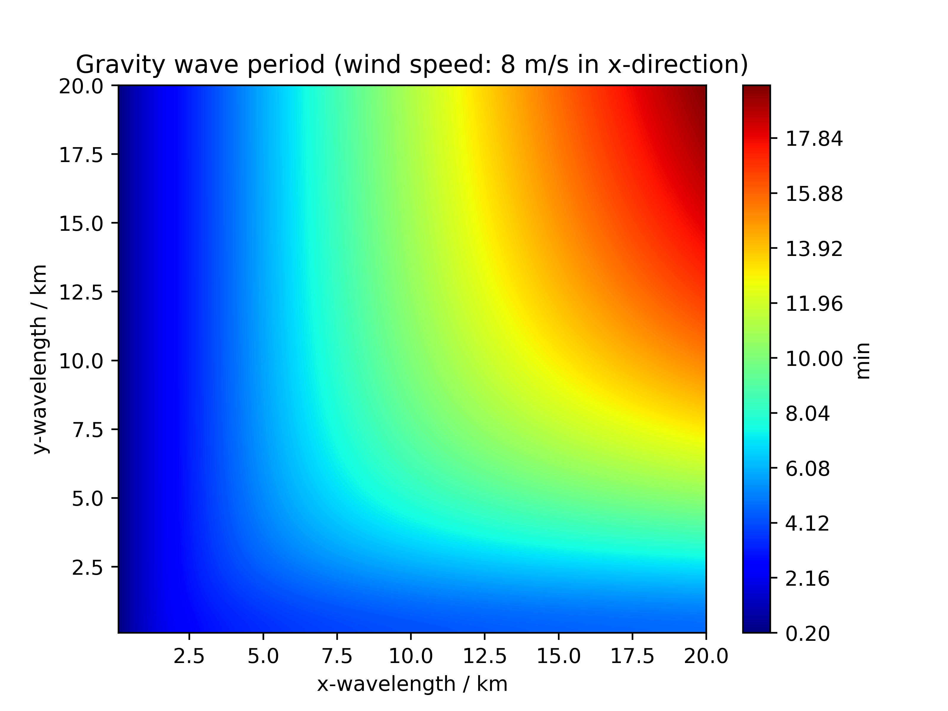
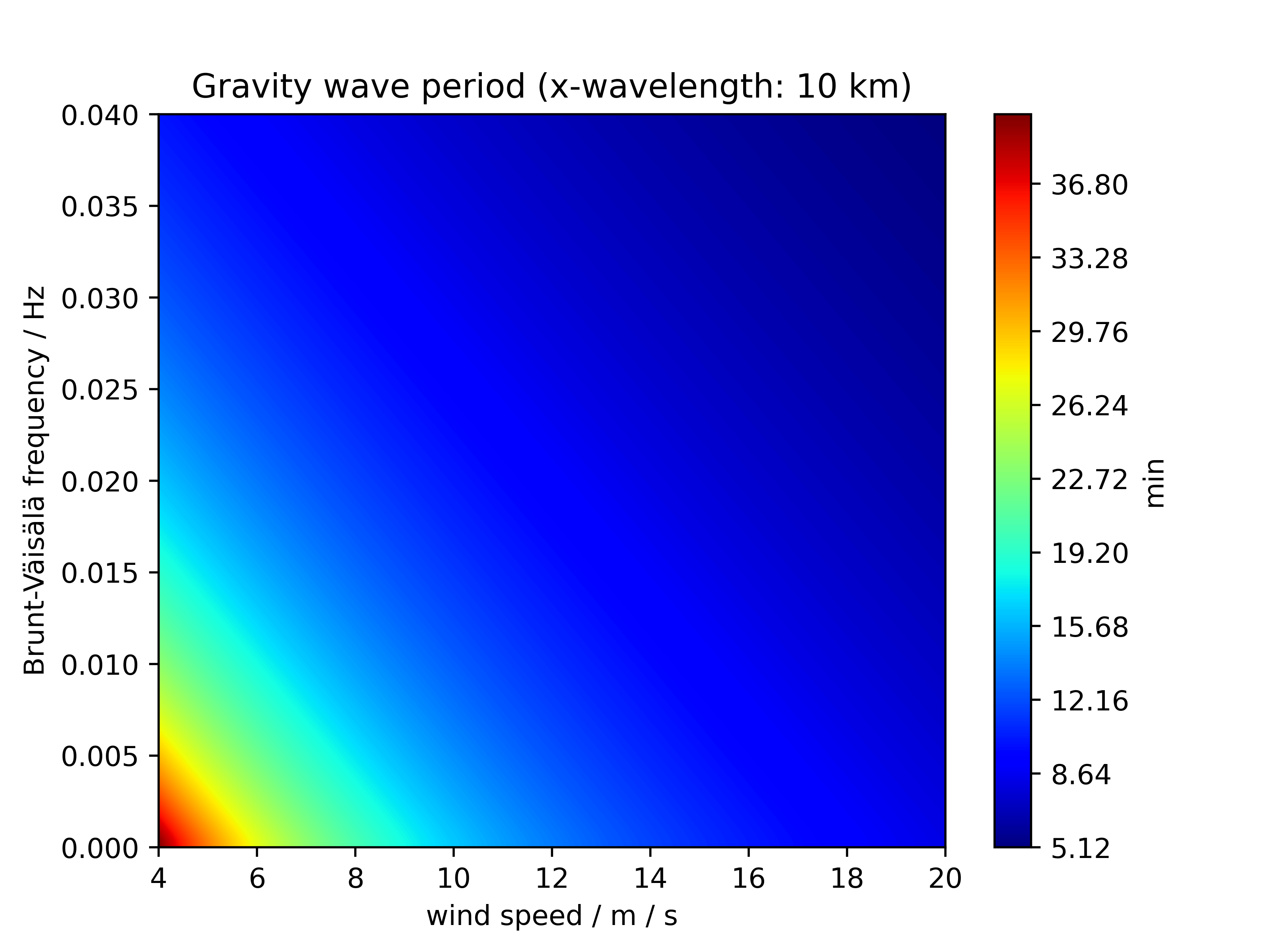
Often one wants to know the period of the expected oscillation as a function of the atmospheric background state $\left(U, N\right)$. The period assuming that the wave vector is parallel to the background wind is shown in Fig. 16.5.

16.6.2.1 Limiting cases

For $k^2 + l^2 \to 0$ (waves that do not propagate horizontally relative to the base current) one obtains inertial waves from Eq. (16.242):

For $m^2 + \frac{1}{4H^2} \to \infty$ one gets from Eq. (16.242) oscillations with frequency $N$:

$H \to \infty$ can be interpreted as neglecting vertical density fluctuations. $m \to 0$ means that the wave vector is oriented purely horizontally. These waves arise in a continuous, thermally stable medium when a particle is deflected vertically. A particle of density $\rho _0 = \rho (z_0)$ has its rest position at the height $z_0$, which is set here to $z_0 = 0$ without loss of generality. If one deflects the particle vertically, the equation of motion reads:

\[ \begin{align} \frac{d^2z}{dt^2} = -\frac{1}{\rho_0}\frac{\partial p}{\partial z} - g = g\frac{\rho}{\rho_0} - g = \frac{g}{\rho_0}\left(\rho - \rho_0\right), \tag{16.245}\label{eq:momentum_schichtung} \end{align} \]

Let $z(t)$ be the deflection. It was assumed that the particle does not change its density during the deflection. If one approximates the deviation $\rho (z) - \rho _0$ by a Taylor expansion

\[ \begin{align} \rho\left(t\right) - \rho_0 = \frac{\partial\rho}{\partial z}(z = 0)z, \end{align} \]

then it follows for the oscillation equation

\[ \begin{align} \frac{d^2z}{dt^2}(t) = \frac{g}{\rho_0}\frac{\partial\rho}{\partial z}z(t)\tag{16.247}\label{eq:schichtungs_dg}. \end{align} \]

Making the ansatz $z = Z_1\exp\left(iNt\right) + Z_2\exp\left(-iNt\right)$, it follows for the angular frequency

\[ \begin{align} N^2 = -\frac{g}{\rho}\frac{\partial\rho}{\partial z}, \end{align} \]

$N$ is the Brunt-Väisälä frequency, it is a measure of stability. Substituting $N$ into Eq. (16.247), one obtains

\[ \begin{align} \frac{d^2z}{dt^2} = -N^2z. \end{align} \]

This shows that in the case $N^2 > 0$ a sinusoidal oscillation results as the solution, while in the case $N^2 < 0$ a real exponential function is the solution, since the particle is accelerated away from its original position. In the case $N^2> 0$ the stratification is stable, while in the case $N^2<0$ it is unstable. Stable stratification is also referred to as strong stratification. In the case $N^2 = 0$ the stratification is neutral.

The above derivation is not yet entirely complete, since incompressibility was assumed. Strictly speaking, it is not the density that is conserved during the deflection, but rather the potential density relative to the reference level. If $\newtilde{\rho}(z)$ denotes the density of the particle at a deflection $z$, then Eq. (16.245) becomes

\[ \begin{align} \frac{d^2z}{dt^2} = \frac{1}{\newtilde{\rho}\left(z\right)}g\rho\left(z\right) - g = \frac{g}{\newtilde{\rho}\left(z\right)} \left(\rho\left(z\right) - \newtilde{\rho}\left(z\right)\right). \end{align} \]

The expression $\rho\left(z\right) - \newtilde{\rho}\left(z\right)$ is the density difference between the surrounding fluid and the particle under consideration. If one brings both systems adiabatically to $z = 0$, then according to Eq. (9.44) one has for their density difference

\[ \begin{align} \Delta\rho = \left(\rho\left(z\right) - \newtilde{\rho}\left(z\right)\right)\left(\frac{p_0}{p}\right)^{1/\kappa}. \end{align} \]

Here $p \coloneqq p\left(z\right)$ and $p_0 \coloneqq p\left(0\right)$. To first order, $p = p_0$; $\Delta\rho$ is then the difference of the potential densities with respect to the reference level $z = 0$. Therefore one can also use the potential densities $\rho_\theta$ (referred to $z = 0$). One obtains, to first order,

\[ \begin{align} \frac{d^2z}{dt^2} = \frac{g}{\newtilde{\rho}(z)}\left(\rho_\theta(z) - \rho_\theta\left(0\right)\right) = \frac{g}{\newtilde{\rho}(z)}\frac{\partial\rho_\theta}{\partial z}z. \end{align} \]

For the Brunt-Väisälä frequency, it follows that

This is the general expression for the Brunt-Väisälä frequency in a compressible medium. $N^2$ is a field that can depend on all three coordinates and time. The potential density must always be referred to the level at which one is located. In a dry atmosphere $N^2$ can also be expressed in terms of the potential temperature $\theta$:

\[ \begin{align} \rho_\theta = \frac{p_0}{R_d\theta} \end{align} \]

It thus follows that

\[ \begin{align} \frac{\partial\rho_\theta}{\partial z} = -\frac{p_0}{R_d\theta^2}\frac{\partial\theta}{\partial z}. \end{align} \]

For the Brunt-Väisälä frequency, this means

\[ \begin{align} N^2 &= \frac{g}{\theta}\frac{\partial\theta}{\partial z}.\tag{16.256}\label{eq:bv_freq_theta} \end{align} \]

Such waves, also referred to as buoyancy oscillations, arise, for example, as lee waves behind orography; in this case sinusoidal trajectories $(ut, z_0\sin\left(Nt\right))^T$ result. When saturation is reached, clouds form in the wave crests.

16.6.2.2 Hydrostatic gravity waves

Neglecting the blue terms in Eq. (16.242) provides the dispersion relation of hydrostatic gravity waves:

16.6.2.3 Group velocity

From this equation, it follows that

\[ \begin{align} \nabla_\mathbf{k}\omega_I^2 = \left(\begin{array}{c} \frac{2N^2k}{m^2 + \frac{1}{4H^2}}\\ \frac{2N^2l}{m^2 + \frac{1}{4H^2}}\\ -2m\frac{N^2\left(k^2 + l^2\right)}{\left(m^2 + \frac{1}{4H^2}\right)^2} \end{array}\right). \end{align} \]

With $\omega' = \sign\left(\omega\right)\sqrt{\omega^2}' = \frac{1}{2\omega}\left(\omega^2\right)'$ one obtains for the group velocity of hydrostatic baroclinic gravity waves

\[ \begin{align} \mathbf{c}_\text{gr} = \frac{1}{\omega_I}\left(\begin{array}{c} \frac{N^2k}{m^2 + \frac{1}{4H^2}}\\ \frac{N^2l}{m^2 + \frac{1}{4H^2}}\\ -m\frac{N^2\left(k^2 + l^2\right)}{\left(m^2 + \frac{1}{4H^2}\right)^2} \end{array}\right) = \frac{1}{\omega_I}\frac{N^2}{m^2 + \frac{1}{4H^2}}\left(\begin{array}{c} k\\ l\\ -m\frac{k^2 + l^2}{m^2 + \frac{1}{4H^2}} \end{array}\right). \end{align} \]

Horizontally, the group velocity points in the same direction as the phase velocity. Vertically, the two velocities have opposite signs. For the vertical wavelength $l_z$, one has

\[ \begin{align} m^2 = \frac{4\pi^2}{l_z^2} \Rightarrow \frac{m^2}{\frac{1}{4H^2}} = \frac{16\pi^2H^2}{l_z^2} \approx 158\frac{H^2}{l_z^2}. \end{align} \]

Often, one has

\[ \begin{align} \frac{m^2}{\frac{1}{4H^2}} \gg 1. \end{align} \]

Under this condition, one has

\[ \begin{align} \mathbf{c}_\text{gr} &= \frac{\sign\left(\omega_I\right)}{\sqrt{f^2 + \frac{N^2}{m^2}\left(k^2 + l^2\right)}}\frac{N^2}{m^2}\left(\begin{array}{c} k\\ l\\ -\frac{k^2 + l^2}{m} \end{array}\right) = \frac{\sign\left(\omega_I\right)}{\sqrt{f^2m^2 + N^2\left(k^2 + l^2\right)}}\frac{N^2}{m}\left(\begin{array}{c} k\\ l\\ -\frac{k^2 + l^2}{m} \end{array}\right)\\ \Rightarrow\mathbf{c}_\text{gr}\cdot\mathbf{k} &\propto k^2 + l^2 - \left(k^2 + l^2\right) = 0. \end{align} \]

Phase velocity and group velocity are therefore perpendicular to each other.

16.6.2.4 Amplitude behavior

From the Bretherton transformation Eqs. (16.225) - (16.226) and Eq. (16.229), it follows that

\[ \begin{align} u' \coloneqq \sqrt{\frac{\rho_\text{SFC}}{\rho_0}}u'' = \exp\left(\frac{z}{2H}\right)u'', & {} & v' \coloneqq \sqrt{\frac{\rho_\text{SFC}}{\rho_0}}v'' = \exp\left(\frac{z}{2H}\right)v'',\\ w' \coloneqq \sqrt{\frac{\rho_\text{SFC}}{\rho_0}}w'' = \exp\left(\frac{z}{2H}\right)w'', & {} & p' \coloneqq \sqrt{\frac{\rho_0}{\rho_\text{SFC}}}p'' = \exp\left(-\frac{z}{2H}\right)p''. \end{align} \]

The amplitude of the motions thus increases exponentially with height, while the magnitude of the pressure fluctuations decreases exponentially.

16.6.2.5 Lee waves

Lee waves are stationary, i.e. $\omega = 0$. From this it follows

\[ \begin{align} \omega_I = \omega - Uk = -Uk\Rightarrow \omega_I^2 = U^2k^2. \end{align} \]

Assuming hydrostatic gravity waves and using Eq. (16.257), one obtains

\[ \begin{align} \omega_I^2 = U^2k^2 &= f^2 + \frac{N^2\left(k^2 + l^2\right)}{m^2 + \frac{1}{4H^2}}. \end{align} \]

Assuming $m^2 \gg \frac{1}{4H^2}$, $f = 0$ and $l = 0$, it follows

\[ \begin{align} \omega_I^2 = U^2k^2 = \frac{N^2k^2}{m^2}\Rightarrow U^2 &= \frac{N^2}{m^2} \Rightarrow m^2 = \frac{N^2}{U^2}. \end{align} \]

This follows for the intrinsic phase velocity

\[ \begin{align} \mathbf{c}_{I, \text{ph}} = \frac{\omega_I}{\sqrt{k^2 + m^2}}\frac{\mathbf{k}}{\left|\mathbf{k}\right|} = -\frac{Uk}{k^2 + m^2}\left( \begin{array}{c} k\\ 0\\ m \end{array} \right) \end{align} \]

as well as for the intrinsic group velocity

\[ \begin{align} \mathbf{c}_{I, \text{gr}} = \nabla_\mathbf{k}\omega_I = \left( \begin{array}{c} -\frac{N}{m}\\ 0\\ \frac{Nk}{m^2} \end{array} \right). \end{align} \]

The intrinsic phase velocity is directed downwards and against the wind direction, the intrinsic group velocity is also negative in the x direction, but directed upwards.

In the case of non-hydrostatic gravity waves, one has with Eq. (16.242), again under the assumptions $f = 0$ and $l = 0$,

\[ \begin{align} U^2k^2 &= \frac{N^2k^2}{m^2 + \frac{1}{4H^2} + k^2} \Leftrightarrow U^2\left(k^2 + m^2 + \frac{1}{4H^2}\right) = N^2\nonumber\\ \Leftrightarrow m^2 &= \frac{N^2}{U^2} - k^2 - \frac{1}{4H^2}. \end{align} \]

In the case $m^2 < 0$ the waves are vertically evanescent, so they cannot propagate vertically. This is the case for

\[ \begin{align} \frac{N^2}{U^2} - k^2 - \frac{1}{4H^2} < 0 & {} & \Leftrightarrow k^2 > \frac{N^2}{U^2} - \frac{1}{4H^2}\nonumber\\ \Leftrightarrow \frac{4\pi^2}{l_x^2} > \frac{N^2}{U^2} - \frac{1}{4H^2} & {} & \Leftrightarrow \frac{l_x^2}{4\pi^2} < \frac{1}{\frac{N^2}{U^2} - \frac{1}{4H^2}}\nonumber\\ \Leftrightarrow l_x < \frac{2\pi}{\sqrt{\frac{N^2}{U^2} - \frac{1}{4H^2}}}.& {} & \end{align} \]

Those spectral components of the orography that fulfill this inequality cannot generate upward propagating waves. Substituting typical values of $N = 0.02$ Hz, $U = 8$ m/s and $H = 8$ km gives $l_x \approx 2.5$ km. With higher wind speed, $l_x$ increases.

16.6.3 Rossby waves

In order to understand so-called Rossby waves, one uses the quasi-geostrophic equation system derived in Sect. 13.11, consisting of the tendency equation Eq. (13.226) and the $\omega-$equation Eq. (13.231), but here in discretized form. The prognostic (state-determining) variables here are two stream functions $\psi_1$, $\psi_3$. The resulting five layers are summarized in Tab. 16.1. The boundary conditions $\omega_0 = \omega_4 = 0$ are used for calculation.

Overview of the quasi-geostrophic two-layer model. See [26].

Index	Pressure / hPa	defined function
$0$	$0$	$\omega_0 = 0$ (boundary condition)
$1$	$250$	$\psi_1$
$2$	$500$	$\omega_2$
$3$	$750$	$\psi_3$
$4$	$1000$	$\omega_4 = 0$ (boundary condition)

This ansatz is called the quasigeostrophic two-layer model.

For the quasi-geostrophic potential vorticities, one has

\[ \begin{align} q_1 &= f + \Delta\psi_1 + \frac{f_0^2}{\sigma}\frac{\frac{\partial\psi}{\partial p}\newvline_{_2} - \frac{\partial\psi}{\partial p}\newvline_{_0}}{\Delta p} = f + \Delta\psi_1 + \frac{f_0^2}{\sigma\Delta p^2}\left(\psi_3 - \psi_1\right) - \frac{f_0^2\frac{\partial\psi}{\partial p}\newvline_{_0}}{\sigma\Delta p},\\ q_3 &= f + \Delta\psi_3 + \frac{f_0^2}{\sigma}\frac{\frac{\partial\psi}{\partial p}\newvline_{_4} - \frac{\partial\psi}{\partial p}\newvline_{_2}}{\Delta p} = f + \Delta\psi_3 - \frac{f_0^2}{\sigma\Delta p^2}\left(\psi_3 - \psi_1\right) + \frac{f_0^2\frac{\partial\psi}{\partial p}\newvline_{_4}}{\sigma\Delta p}. \end{align} \]

Here $\Delta p \coloneqq500$ hPa is defined. No statement can be made about the last terms within the framework of this model, so they are assumed constant and thus neglected. One further defines a barotropic and a baroclinic component of the stream function:

\[ \begin{align} \psi_M \coloneqq&\frac{\psi_1 + \psi_3}{2}, & {} & \psi_T \coloneqq \frac{\psi_1 - \psi_3}{2}. \end{align} \]

In addition, a baroclinic potential vorticity is defined:

\[ \begin{align} q_T \coloneqq\frac{q_1 - q_3}{2} = \frac{\zeta_1 - \zeta_3}{2} - \frac{f_0^2}{\sigma\Delta p^2}\left(\psi_1 - \psi_3\right) \end{align} \]

Furthermore, the stability wave number $K$ is given by

\[ \begin{align} K^2 \coloneqq\frac{2f_0^2}{\sigma\Delta p^2} \end{align} \]

defined. This allows one to write

\[ \begin{align} q_1 = f + \zeta_1 - K^2\psi_T, & {} & q_3 = f + \zeta_3 + K^2\psi_T, & {} & q_T = \zeta_T - K^2\psi_T. \end{align} \]

Now one makes a perturbation ansatz

\[ \begin{align} \psi = \newoverline{\psi} + \psi' = -\newoverline{u}y + \psi' \end{align} \]

with a mean homogeneous zonal flow vector $\newoverline{u}$. Now one assumes a special case: one assumes that at level 1 the background wind

\[ \begin{align} \newoverline{u}_1 = \newoverline{u}_T \end{align} \]

blows, and at level 3 the background wind

\[ \begin{align} \newoverline{u}_3 = -\newoverline{u}_T. \end{align} \]

The following then hold

\[ \begin{align} \newoverline{\psi}_1 = -\newoverline{u}_Ty, & {} & \newoverline{\psi}_3 = \newoverline{u}_Ty. \end{align} \]

From this it follows

\[ \begin{align} \newoverline{\psi}_T &= -\newoverline{u}_Ty. \end{align} \]

For the basic state $\newoverline{\mathbf{v}_h}$, one can thus write

\[ \begin{align} \newoverline{\mathbf{v}_h}_1 &= \left(\begin{array}{c} \newoverline{u}_T\\ 0 \end{array}\right),\\ \newoverline{\mathbf{v}_h}_3 &= \left(\begin{array}{c} - \newoverline{u}_T\\ 0 \end{array}\right). \end{align} \]

Let the field $\newoverline{u}_T$ be independent of $y$; then one has

\[ \begin{align} \newoverline{\zeta}_1 = \newoverline{\zeta}_3 = 0. \end{align} \]

For the potential vorticities, one has

\[ \begin{align} \newoverline{q}_1 &= f_0 + \beta y - K^2\newoverline{\psi}_T = f_0 + \left(\beta + K^2\newoverline{u}_T\right)y,\\ \newoverline{q}_3 &= f_0 + \beta y + K^2\newoverline{\psi}_T = f_0 + \left(\beta - K^2\newoverline{u}_T\right)y. \end{align} \]

This field is stationary:

\[ \begin{align} \left(\frac{\partial}{\partial t} + \newoverline{\mathbf{v}_h}_1\cdot\nabla\right)\newoverline{q}_1 &= 0\\ \left(\frac{\partial}{\partial t} + \newoverline{\mathbf{v}_h}_3\cdot\nabla\right)\newoverline{q}_3 &= 0 \end{align} \]

If one also applies the perturbation ansatz to the form of the material derivative used here and to the potential vorticity, it follows

\[ \begin{align} \md{_h^{(g)}} &= \frac{\partial}{\partial t} + \newoverline{\mathbf{v}_h}\cdot\nabla + \mathbf{v}_h'\cdot\nabla,\\ q &= \newoverline{q} + q'. \end{align} \]

Now one again assumes that the perturbations have only meridional components, i.e.

\[ \begin{align} \mathbf{v}_{h, g, 1}' &= \left(\begin{array}{c} 0\\ v_1' \end{array}\right),\\ \mathbf{v}_{h, g, 3}' &= \left(\begin{array}{c} 0\\ v_3' \end{array}\right). \end{align} \]

For the stream functions, one has

\[ \begin{align} v_1' = \frac{\partial\psi_1'}{\partial x}, & {} & v_3' = \frac{\partial\psi_3'}{\partial x}. \end{align} \]

From this it follows for the potential vorticities

\[ \begin{align} q_1' = \frac{\partial^2\psi_1'}{\partial x^2} - K^2\psi_T', & {} & q_3' = \frac{\partial^2\psi_3'}{\partial x^2} + K^2\psi_T'. \end{align} \]

To examine the tendency equations, one writes

\[ \begin{align} \frac{\partial\newoverline{q}}{\partial t} + \newoverline{\mathbf{v}_h}\cdot\nabla\newoverline{q} + \frac{\partial q'}{\partial t} + \newoverline{\mathbf{v}_h}\cdot\nabla q' + \mathbf{v}_h'\cdot\nabla\newoverline{q} + \mathbf{v}_h'\cdot\nabla q' = 0. \end{align} \]

The first two terms give zero, as already noted. The last scalar product also vanishes owing to the orthogonality of the vectors involved. Thus, the following hold

\[ \begin{align} \left(\frac{\partial}{\partial t} + \newoverline{u}_T\frac{\partial}{\partial x}\right)q_1' + \left(\beta + K^2\newoverline{u}_T\right)\frac{\partial\psi_1'}{\partial x} &= 0, \tag{16.298}\label{eq:dgl_baroklin_1}\\ \left(\frac{\partial}{\partial t} - \newoverline{u}_T\frac{\partial}{\partial x}\right)q_3' + \left(\beta - K^2\newoverline{u}_T\right)\frac{\partial\psi_3'}{\partial x} &= 0.\tag{16.299}\label{eq:dgl_baroklin_2} \end{align} \]

Since Eqs. (16.298) - (16.299) are linear, one can regard the solutions as superpositions of plane waves and therefore makes an ansatz

\[ \begin{align} \psi_1' &= A_1\exp\left[i\left(kx - \omega t\right)\right] = :A_1f\left(x, t\right),\\ \psi_3' &= A_3\exp\left[i\left(kx - \omega t\right)\right] = :A_3f\left(x, t\right). \end{align} \]

One thus obtains

\[ \begin{align} q_1' &= -k^2A_1f - K^2\frac{A_1 - A_3}{2}f,\\ q_3' &= -k^2A_3f + K^2\frac{A_1 - A_3}{2}f. \end{align} \]

The system of equations to be solved is thus

\[ \begin{align} \left(\omega - k\newoverline{u}_T\right)\left(k^2A_1 + K^2\frac{A_1 - A_3}{2}\right) + \left(\beta + K^2\newoverline{u}_T\right)kA_1 &= 0,\\ \left(\omega + k\newoverline{u}_T\right)\left(k^2A_3 - K^2\frac{A_1 - A_3}{2}\right) + \left(\beta - K^2\newoverline{u}_T\right)kA_3 &= 0. \end{align} \]

In matrix notation, this reads:

\[ \begin{align} \left(\begin{array}{cc} M_{1, 1}&M_{1, 2}\\ M_{2, 1}&M_{2, 2} \end{array}\right)\left(\begin{array}{c} A_1\\ A_3 \end{array}\right) = \mathbf{0} \end{align} \]

with the matrix coefficients

\[ \begin{align} M_{1, 1} &= \left(\omega - k\newoverline{u}_T\right)\left(k^2 + \frac{K^2}{2}\right) + \left(\beta + K^2\newoverline{u}_T\right)k,\\ M_{1, 2} &= -\frac{K^2}{2}\left(\omega - k\newoverline{u}_T\right),\\ M_{2, 1} &= -\frac{K^2}{2}\left(\omega + k\newoverline{u}_T\right),\\ M_{2, 2} &= \left(\omega + k\newoverline{u}_T\right)\left(k^2 + \frac{K^2}{2}\right) + \left(\beta - K^2\newoverline{u}_T\right)k. \end{align} \]

Setting the determinant to zero yields

\[ \begin{align} & M_{1, 1}M_{2, 2} - M_{2, 1}M_{1, 2}\hastobe0\nonumber\\ &\Rightarrow\left(\omega^2 - k^2\newoverline{u}_T^2\right)\left(k^2 + \frac{K^2}{2}\right)^2 + 2k\left(k^2 + \frac{K^2}{2}\right)\left(\omega\beta + kK^2\newoverline{u}_T^2\right) + \left(\beta^2 - K^4\newoverline{u}_T^2\right)k^2 - \frac{K^4}{4}\left(\omega^2 - k^2\newoverline{u}_T^2\right) = 0\nonumber\\ &\Rightarrow\left(\omega^2 - k^2\newoverline{u}_T^2\right)\left(k^4 + k^2K^2\right) + 2k\left(k^2 + \frac{K^2}{2}\right)\left(\omega\beta + kK^2\newoverline{u}_T^2\right) + \left(\beta^2 - K^4\newoverline{u}_T^2\right)k^2 = 0\nonumber\\ &\Rightarrow\left(\omega^2 - k^2\newoverline{u}_T^2\right)\left(k^2 + K^2\right) + \left(2k + \frac{K^2}{k}\right)\left(\omega\beta + kK^2\newoverline{u}_T^2\right) + \beta^2 - K^4\newoverline{u}_T^2 = 0\nonumber\\ &\Rightarrow\left(\omega^2 - k^2\newoverline{u}_T^2\right)\left(k^2 + K^2\right) + 2k\left(\omega\beta + kK^2\newoverline{u}_T^2\right) + \frac{K^2\omega\beta}{k} + \beta^2 = 0\nonumber\\ &\Rightarrow\omega^2k^2 + \omega^2K^2 - k^4\newoverline{u}_T^2 + k^2K^2\newoverline{u}_T^2 + 2k\omega\beta + \frac{K^2\omega\beta}{k} + \beta^2 = 0\nonumber \end{align} \] \[ \begin{align} &\Rightarrow\omega^2\left[k^2 + K^2\right] + \omega\left[2k\beta + \frac{K^2\beta}{k}\right] - k^4\newoverline{u}_T^2 + k^2K^2\newoverline{u}_T^2 + \beta^2 = 0\nonumber\\ &\Rightarrow\omega^2 + \omega\frac{\beta}{k}\frac{2k^2 + K^2}{k^2 + K^2} + \frac{k^2K^2\newoverline{u}_T^2 - k^4\newoverline{u}_T^2 + \beta^2}{k^2 + K^2} = 0\nonumber\\ &\Rightarrow\omega_{1, 2} = -\frac{\beta}{2k}\frac{2k^2 + K^2}{k^2 + K^2}\pm\sqrt{\frac{\beta^2}{4k^2}\frac{\left(2k^2 + K^2\right)^2}{\left(k^2 + K^2\right)^2} - \frac{k^2K^2\newoverline{u}_T^2 - k^4\newoverline{u}_T^2 + \beta^2}{k^2 + K^2}}\nonumber\\ &\Rightarrow\omega_{1, 2} = -\frac{\beta}{2k}\frac{2k^2 + K^2}{k^2 + K^2}\pm\frac{1}{k^2 + K^2}\sqrt{\frac{\beta^2}{4k^2}\left(4k^4 + K^4 + 4k^2K^2\right) - \left(k^2 + K^2\right)\left(k^2K^2\newoverline{u}_T^2 - k^4\newoverline{u}_T^2 + \beta^2\right)}\nonumber\\ &\Rightarrow\omega_{1, 2} = -\frac{\beta}{2k}\frac{2k^2 + K^2}{k^2 + K^2}\nonumber\\ &\pm\frac{1}{k^2 + K^2}\sqrt{\beta^2k^2 + \frac{\beta^2K^4}{4k^2} + \beta^2K^2 - k^4K^2\newoverline{u}_T^2 - k^2\beta^2 - K^4k^2\newoverline{u}_T^2 - K^2\beta^2 + k^6\newoverline{u}_T^2 + K^2k^4\newoverline{u}_T^2}\nonumber\\ &\Rightarrow\omega_{1, 2} = -\frac{\beta}{k}\frac{k^2 + K^2/2}{k^2 + K^2}\pm\frac{1}{k^2 + K^2}\sqrt{\frac{\beta^2K^4}{4k^2} + \newoverline{u}_T^2k^2\left(k^4 - K^4\right)}.\tag{16.311}\label{eq:disp_rel_baroklin} \end{align} \]

Assuming $k < K$, one maximizes the expression under the square root by setting $\newoverline{u}_T = 0$, from which it follows

Baroclinic Rossby waves therefore always propagate westward. Baroclinic Rossby waves, too, are called planetary waves when they span a complete circle of latitude.

16.6.4 Natural oscillations of a hydrostatic atmosphere

One writes the equations summarized in Sect. 13.7.4 in their adiabatic form:

\[ \begin{align} \frac{\partial u}{\partial t} + u\frac{\partial u}{\partial x} + v\frac{\partial u}{\partial y} + \omega\frac{\partial u}{\partial p} &= -\frac{\partial\Phi}{\partial x} + fv,\\ \frac{\partial v}{\partial t} + u\frac{\partial v}{\partial x} + v\frac{\partial v}{\partial y} + \omega\frac{\partial v}{\partial p} &= -\frac{\partial\Phi}{\partial y} - fu,\\ \frac{\partial^2\Phi}{\partial p\partial t} + \left(u\frac{\partial}{\partial x} + v\frac{\partial}{\partial y}\right)\frac{\partial\Phi}{\partial p} + \frac{\alpha^2}{g^2}N^2\omega &= 0,\\ \frac{\partial\omega}{\partial p} &= -\nabla\cdot\mathbf{v}_h. \end{align} \]

Neglecting advection, one obtains

\[ \begin{align} \frac{\partial u}{\partial t} &= -\frac{\partial\Phi}{\partial x} + fv,\\ \frac{\partial v}{\partial t} &= -\frac{\partial\Phi}{\partial y} - fu,\\ \frac{\partial^2\Phi}{\partial p\partial t} + \sigma\omega &= 0,\\ \frac{\partial\omega}{\partial p} &= -\nabla\cdot\mathbf{v}_h. \end{align} \]

with the static stability parameter $\sigma = \frac{\alpha^2}{g^2}N^2$. This is the underlying system of equations for this section. Writing the derivatives and differential operators in geographical coordinates, one obtains

\[ \begin{align} \frac{\partial u}{\partial t} &= -\frac{1}{a\cos\left(\phi\right)}\frac{\partial\Phi}{\partial\lambda} + fv,\tag{16.321}\label{eq:hydrostatic_normal_0}\\ \frac{\partial v}{\partial t} &= -\frac{1}{a}\frac{\partial\Phi}{\partial\phi} - fu,\tag{16.322}\label{eq:hydrostatic_normal_1}\\ \frac{\partial^2\Phi}{\partial p\partial t} + \sigma\omega &= 0,\tag{16.323}\label{eq:hydrostatic_normal_2}\\ \frac{\partial\omega}{\partial p} &= -\frac{1}{a\cos\left(\phi\right)}\frac{\partial u}{\partial\lambda} - \frac{1}{a}\frac{\partial v}{\partial\phi} - \frac{v}{a}\tan\left(\phi\right).\tag{16.324}\label{eq:hydrostatic_normal_3} \end{align} \]

One now performs a decomposition into a background state $\newoverline{\mathbf{\psi}}$ and deviations $\mathbf{\psi}'$, where $\sigma$ is a property of the background state. One assumes $\newoverline{u} = \newoverline{v} = \newoverline{\omega} = 0$. As ansätze for fields $\psi$, one uses

\[ \begin{align} \psi' = \psi_0\left(\frac{p}{p_0}\right)^\chi h\left(\phi\right)\exp\left(im\lambda - i\gamma t\right) \end{align} \]

with a complex amplitude $\psi_0$, a zonal wavenumber $m \in \mathbb{N}$ and a continuously differentiable function $h\left(\phi\right)$. $p_0$ is a reference pressure and $\chi > 0$ is a parameter. Substituting this and the definition of $f$ into Eqs. (16.321) - (16.324), one obtains

\[ \begin{align} -i\gamma u_0 &= -\frac{im\Phi_0}{a\cos\left(\phi\right)} + 2\Omega\sin\left(\phi\right)v_0,\\ -i\gamma hv_0 &= -\frac{\Phi_0 h'}{a} - 2\Omega\sin\left(\phi\right)u_0h,\\ -i\gamma\frac{\chi}{p}\Phi_0 &= -\sigma\omega_0,\\ \frac{\chi}{p}h\omega_0 &= -\frac{imh}{a\cos\left(\phi\right)}u_0 - \frac{v_0h'}{a} - \frac{v_0}{a}h\tan\left(\phi\right). \end{align} \]

The fractions are cleared:

\[ \begin{align} -i\gamma a\cos\left(\phi\right)u_0 &= -im\Phi_0 + 2\Omega a\cos\left(\phi\right)\sin\left(\phi\right)v_0 = -im\Phi_0 + \Omega a\sin\left(2\phi\right)v_0,\\ -i\gamma ahv_0 &= -h'\Phi_0 - 2\Omega a\sin\left(\phi\right)hu_0,\\ -i\gamma\chi\Phi_0 &= -\sigma p\omega_0,\\ \chi ha\cos\left(\phi\right)\omega_0 &= -imhpu_0 - ph'\cos\left(\phi\right)v_0 - ph\sin\left(\phi\right)v_0 \end{align} \]

Bringing everything to the left-hand side, one obtains

\[ \begin{align} -i\gamma a\cos\left(\phi\right)u_0 + im\Phi_0 - \Omega a\sin\left(2\phi\right)v_0 &= 0,\\ -i\gamma ahv_0 + h'\Phi_0 + 2\Omega a\sin\left(\phi\right)hu_0 &= 0,\\ -i\gamma\chi\Phi_0 + \sigma p\omega_0 &= 0,\\ \chi ha\cos\left(\phi\right)\omega_0 + imhpu_0 + ph'\cos\left(\phi\right)v_0 + ph\sin\left(\phi\right)v_0 &= 0. \end{align} \]

The terms are now sorted in the order $u_0$, $v_0$, $\Phi_0$, $\omega_0$:

\[ \begin{align} \begin{array}{ccccc} -i\gamma a\cos\left(\phi\right)u_0 &- \Omega a\sin\left(2\phi\right)v_0 &+ im\Phi_0 &+ 0 &= 0,\\ 2\Omega a\sin\left(\phi\right)hu_0 &- i\gamma ahv_0 &+ h'\Phi_0 &+ 0 &= 0,\\ 0 &+ 0 &-i\gamma\chi\Phi_0 &+ \sigma p\omega_0 &= 0,\\ imhpu_0 &+ \left[ph'\cos\left(\phi\right) + ph\sin\left(\phi\right)\right]v_0 &+ 0 &+ \chi ha\cos\left(\phi\right)\omega_0 &= 0. \end{array} \end{align} \]

This leads directly to matrix notation

\[ \begin{align} M\cdot\mathbf{x} = \mathbf{0} \end{align} \]

with

\[ \begin{align} M \coloneqq \left( \begin{array}{cccc} -i\gamma a\cos\left(\phi\right) & -\Omega a\sin\left(2\phi\right) & im & 0,\\ 2\Omega a\sin\left(\phi\right)h & -i\gamma ah & h' & 0,\\ 0 & 0 & -i\gamma\chi & \sigma p,\\ imhp & ph'\cos\left(\phi\right) + ph\sin\left(\phi\right) & 0 & \chi ha\cos\left(\phi\right) \end{array}\right) \end{align} \]

and

\[ \begin{align} \mathbf{v} \coloneqq \left(\begin{array}{c} u_0\\ v_0\\ \Phi_0\\ \omega_0\end{array}\right). \end{align} \]

16.6.4.1 Atmospheric tide

Important differences between the atmospheric and the oceanic tide (see Sect. 16.5.7) are as follows:

• The oceanic tide can be viewed as barotropic, effects of the ocean's baroclinicity play a minor role.

• In the atmosphere, baroclinicity is much more relevant; the barotropic approximation would filter out essential structural elements of the atmospheric tide.

• The oceanic tide is generated primarily by fluctuations in gravity caused by the Moon. This leads to a base period of just under 25 hours.

• The atmospheric tide is driven primarily by radiation and by processes triggered by radiation (chemical reactions and convection).

• Due to barotropy, the oceanic tide is virtually independent of height, while the amplitude of the atmospheric tide increases exponentially with height. This means that the tide plays a role in the atmosphere, especially in the mesosphere (50 - 80 km), where it can reach large amplitudes. In the troposphere, its amplitude is small.

16.7 Instabilities

If one finds angular frequencies with a positive imaginary part when a plane wave is introduced as a disturbance into a system of equations and subsequent linearization (justified for small amplitudes), then a instability is present. The amplitude of the wave grows exponentially in this initial linear time before nonlinear effects become dominant and cause the wave to break with subsequent dissipation of the kinetic energy.

16.7.1 Stratification instability

Over a given point on the Earth's surface, the atmosphere has the stratification $T = T\left(z\right)$. Usually, one has

\[ \begin{align} \frac{\partial T}{\partial z} < 0, \end{align} \]

for $\frac{\partial T}{\partial z}>0$ one speaks of an inversion. The dry adiabatic temperature gradient is defined according to Eq. (9.47) by

\[ \begin{align} \Gamma_d = \frac{g}{c^{(p)}} \end{align} \]

In the case

\[ \begin{align} \frac{\partial T}{\partial z} < -\Gamma_d \end{align} \]

the stratification is unstable, indeed even unconditionally unstable, since neither a saturated nor an unsaturated air particle deflected from its rest position returns to it.

However, if the air is saturated, the cooling that occurs as a result of the uplift causes condensation or resublimation to occur, releasing phase transition heat. If one deflects the particle vertically at $z$, the lifted condensation level (LCL) $z_\text{LCL}$ results as the height at which it would be saturated; it thus satisfies the equation

\[ \begin{align} p_v^{(S)}\left(T\left(z\right) - \Gamma_d\left(z_{\text{LCL}} - z\right)\right) \equiv p_v\left(z\right)\left(1 - \frac{\Gamma_d\left(z_{\text{LCL}} - z\right)}{T\left(z\right)}\right)^{\frac{g}{R_d\Gamma_d}}. \end{align} \]

During the subsequent further uplift, it is initially assumed that all the water remains in the cloud, which is referred to as a reversible wet adiabat; occasionally the word pseudoadiabatic is used instead of wet adiabatic, since the question of whether this process is adiabatic or not depends on which system one considers: if one regards the air including the condensates as the system, the process is adiabatic, since it exchanges no heat with its surroundings; if, however, one considers only the gas phase, the process is diabatic. In the case of an irreversible wet adiabat, discussed in more detail in Sect. 16.7.1.3, it is assumed instead that all the water rains out. This is now considered. Assume, then, that the air in a particle of volume $V$ and constant mass $m$ consists of a mixture of moist air and the condensation products of one phase, all components being assumed to have the same temperature $T$. With the first law of thermodynamics Eq. (9.10), one obtains

\[ \begin{align} &c^{(V)}\frac{dT}{dz} + p\frac{d}{dz}\frac{1}{\rho} = \frac{1}{\rho}\frac{dq}{dz}\nonumber\\ \Rightarrow\frac{dT}{dz} &= \frac{1}{c^{(V)}}\left[\frac{1}{\rho}\frac{dq}{dz} - p\frac{d}{dz}\frac{1}{\rho}\right] = \frac{1}{\rho c^{(V)}}\left[\frac{dq}{dz} + \frac{p}{\rho}\frac{d\rho}{dz}\right] = -\frac{g}{c^{(V)}}\left[\frac{dq}{dp} + \frac{p}{\rho}\frac{d\rho}{dp}\right].\tag{16.346}\label{eq:feuchtad_deriv_1} \end{align} \]

The basic hydrostatic equation was used here. For the heat output per volume due to the phase transition $dq$, one has

\[ \begin{align} dq = \frac{c_{c}}{v}_hdm_c \end{align} \]

with $m_c$ as the condensed or resublimated mass and $c_{c}$ as the phase transition heat. With the equation of state for water vapor, one has

\[ \begin{align} p_v &= \rho_vR_vT\Rightarrow m_v = \frac{V_vp_v}{R_vT} = \frac{V_hp_v}{R_vT} = \frac{m_hR_hp_v^{(S)}\left(T\right)}{pR_v}\nonumber\\ \Rightarrow dm_c &= -dm_v = \frac{m_hR_hp_v^{(S)}\left(T\right)}{pR_v}\left(\frac{dp}{p} - \frac{dp_v^{(S)}}{p_v^{(S)}} + \frac{dm_c}{m_h}\right)\nonumber\\ \Rightarrow dm_c\left(1 - \frac{R_hp_v^{(S)}\left(T\right)}{pR_v}\right) &= \frac{m_hR_hp_v^{(S)}\left(T\right)}{pR_v}\left(\frac{dp}{p} - \frac{dp_v^{(S)}}{p_v^{(S)}}\right)\nonumber\\ \Rightarrow dm_c &= m_h\frac{\frac{dp}{p} - \frac{dp_v^{(S)}}{p_v^{(S)}}}{\frac{pR_v}{R_hp_v^{(S)}} - 1}. \end{align} \]

Here $p_v^{(S)} = p_v^{(S)}\left(T\right)$ is the saturation vapor pressure. From this it follows

\[ \begin{align} dq &= \frac{c_c}{T}\frac{dp - \frac{p}{p_v^{(S)}}dp_v^{(S)}}{\frac{pR_v}{p_v^{(S)}} - R_h}\nonumber\\ \Rightarrow\frac{dq}{dp} &= \frac{c_c}{\frac{pR_vT}{p_v^{(S)}} - R_hT}\left(1 - \frac{p}{p_v^{(S)}}\frac{dp_v^{(S)}}{dp}\right) = \frac{c_c}{\frac{pR_vT}{p_v^{(S)}} - TR_h}\left(1 + \frac{1}{g\rho}\frac{dT}{dz}\frac{p}{p_v^{(S)}}\frac{dp_v^{(S)}}{dT}\right)\nonumber\\ &= \frac{c_c}{TpR_v - Tp_v^{(S)}R_h}\left(p_v^{(S)} + \frac{p}{g\rho}\frac{dT}{dz}\frac{dp_v^{(S)}}{dT}\right)\nonumber\\ &= \frac{c_cp_v^{(S)}}{TpR_v - Tp_v^{(S)}R_h} + \frac{p}{Tg\rho}\frac{c_c}{pR_v - p_v^{(S)}R_h}\frac{dp_v^{(S)}}{dT}\frac{dT}{dz}. \end{align} \]

Putting this into Eq. (16.346) and applying the chain rule once more, one obtains

\[ \begin{align} \frac{dT}{dz} &= -\frac{g}{c^{(V)}}\Bigg[\frac{c_cp_v^{(S)}}{TpR_v - Tp_v^{(S)}R_h}\nonumber\\ & + \frac{p}{Tg\rho}\frac{c_c}{pR_v - p_v^{(S)}R_h}\frac{dp_v^{(S)}}{dT}\frac{dT}{dz} + \frac{p}{\rho}\frac{\partial\rho}{\partial p} - \frac{p}{g\rho^2}\frac{\partial\rho}{\partial T}\frac{dT}{dz}\Bigg]. \end{align} \]

Now one needs an equation of state. For the density, one has

\[ \begin{align} \rho = \rho_h + \rho_c = \frac{p}{R_hT} + \rho_c. \end{align} \]

One thus obtains

\[ \begin{align} \frac{dT}{dz} &= \frac{g}{c^{(V)}}\Bigg[ - \frac{c_cp_v^{(S)}}{TpR_v - Tp_v^{(S)}R_h}\nonumber\\ & - \frac{p}{Tg\rho}\frac{c_c}{pR_v - p_v^{(S)}R_h}\frac{dp_v^{(S)}}{dT}\frac{dT}{dz} - \frac{p}{\rho R_hT} - \frac{p^2}{R_hg\rho^2T^2}\frac{dT}{dz}\Bigg]\nonumber\\ &= \frac{g}{c^{(V)}}\Bigg[ - \frac{c_cp_v^{(S)}}{TpR_v - Tp_v^{(S)}R_h} - \frac{p}{Tg\rho}\frac{c_c}{pR_v - p_v^{(S)}R_h}\frac{dp_v^{(S)}}{dT}\frac{dT}{dz}\nonumber\\ & - 1 + \frac{\rho _c}{\rho} - \frac{1}{g}\left(1 - \frac{\rho_c}{\rho}\right)\frac{p}{\rho T}\frac{dT}{dz}\Bigg]. \end{align} \]

This is now solved for $\frac{dT}{dz}$:

\[ \begin{align} & \frac{dT}{dz}\left(1 + \frac{p}{Tc^{(V)}\rho}\frac{c_c}{pR_v - p_v^{(S)}R_h}\frac{dp_v^{(S)}}{dT} + \frac{1}{c^{(V)}}\left(1 - \frac{\rho_c}{\rho}\right)\frac{p}{\rho T}\right)\nonumber\\ &= \frac{g}{c^{(V)}}\left(\frac{\rho_c}{\rho} - 1\right) - \frac{gc_cp_v^{(S)}\left(T\right)}{c^{(V)}T\left(R_vp - p_v^{(S)}R_h\right)}\nonumber\\ \Rightarrow\frac{dT}{dz} &= -\frac{g}{c^{(p)}}\frac{1 - \frac{\rho_c}{\rho} + \frac{c_cp_v^{(S)}}{T\left(R_vp - p_v^{(S)}R_h\right)}}{\frac{c^{(V)}}{c^{(p)}} + \frac{p}{T\rho c^{(p)}}\frac{c_c}{pR_v - p_v^{(S)}R_h}\frac{dp_v^{(S)}}{dT} + \left(1 - \frac{\rho_c}{\rho}\right)\frac{p}{c^{(p)}T\rho}}\nonumber\\ &= -\Gamma_d\beta \end{align} \]

Here,

The Clausius-Clapeyron equation can be used for the derivative $\frac{dp_v^{(S)}}{dT}$. The so-called moist adiabatic temperature gradient is now defined by

\[ \begin{align} \Gamma_h\coloneqq\Gamma_d\beta \end{align} \]

If one substitutes $\rho_c = 0$ and $p_v \ll p$ into Eq. (16.354) but keeps terms with $\frac{dp_v^{(S)}}{dT}$, it follows

\[ \begin{align} \frac{dT}{dz} &= -\frac{g}{c^{(p)}}\frac{1 + \frac{c_cp_v^{(S)}}{TR_vp}}{\frac{c^{(V)}}{c^{(p)}} + \frac{p}{T\rho c^{(p)}}\frac{c_c}{pR_v}\frac{dp_v^{(S)}}{dT} + \frac{p}{c^{(p)}T\rho}}. \end{align} \]

If one inserts here the equation of state of ideal gases $p = \rho R_dT$, one obtains the expression frequently found in the literature

\[ \begin{align} \frac{dT}{dz} &= -\frac{g}{c^{(p)}}\frac{1 + \frac{c_cp_v^{(S)}}{TR_vp}}{\frac{c^{(V)}}{c^{(p)}} + \frac{R_d}{c^{(p)}}\frac{c_c}{pR_v}\frac{dp_v^{(S)}}{dT} + \frac{c^{(p)} - c^{(V)}}{c^{(p)}}}\nonumber\\ \Leftrightarrow\frac{dT}{dz} &= -\frac{g}{c^{(p)}}\frac{1 + \frac{c_cp_v^{(S)}}{TR_vp}}{1 + \frac{R_dc_c}{R_vc^{(p)}p}\frac{dp_v^{(S)}}{dT}} \equiv -\Gamma_d\beta' \end{align} \]

with a simplified factor

\[ \begin{align} \beta'&= \beta'\left(p, T\right) \coloneqq\frac{1 + \frac{c_cp_v^{(S)}}{TR_vp}}{1 + \frac{\frac{M_v}{M_d}c_c}{pc^{(p)}}\frac{dp_v^{(S)}}{dT}}\stackrel{\href{ch-04-statistical-physics.html#eq:clausius-clapeyron_vereinfacht}{\text{Eq. (5.237)}}}{\approx}\frac{1 + \frac{c_cp_v^{(S)}}{TR_vp}}{1 + \frac{\frac{M_v}{M_d}c_c^2p_v^{(S)}}{R_vc^{(p)}T^2p}}\nonumber \end{align} \]

which no longer depends on the density of the water that has already condensed out. In the case $\frac{dp_v^{(S)}}{dT} = p_v^{(S)} = 0$ it follows

\[ \begin{align} \Gamma_h = \Gamma_d. \end{align} \]

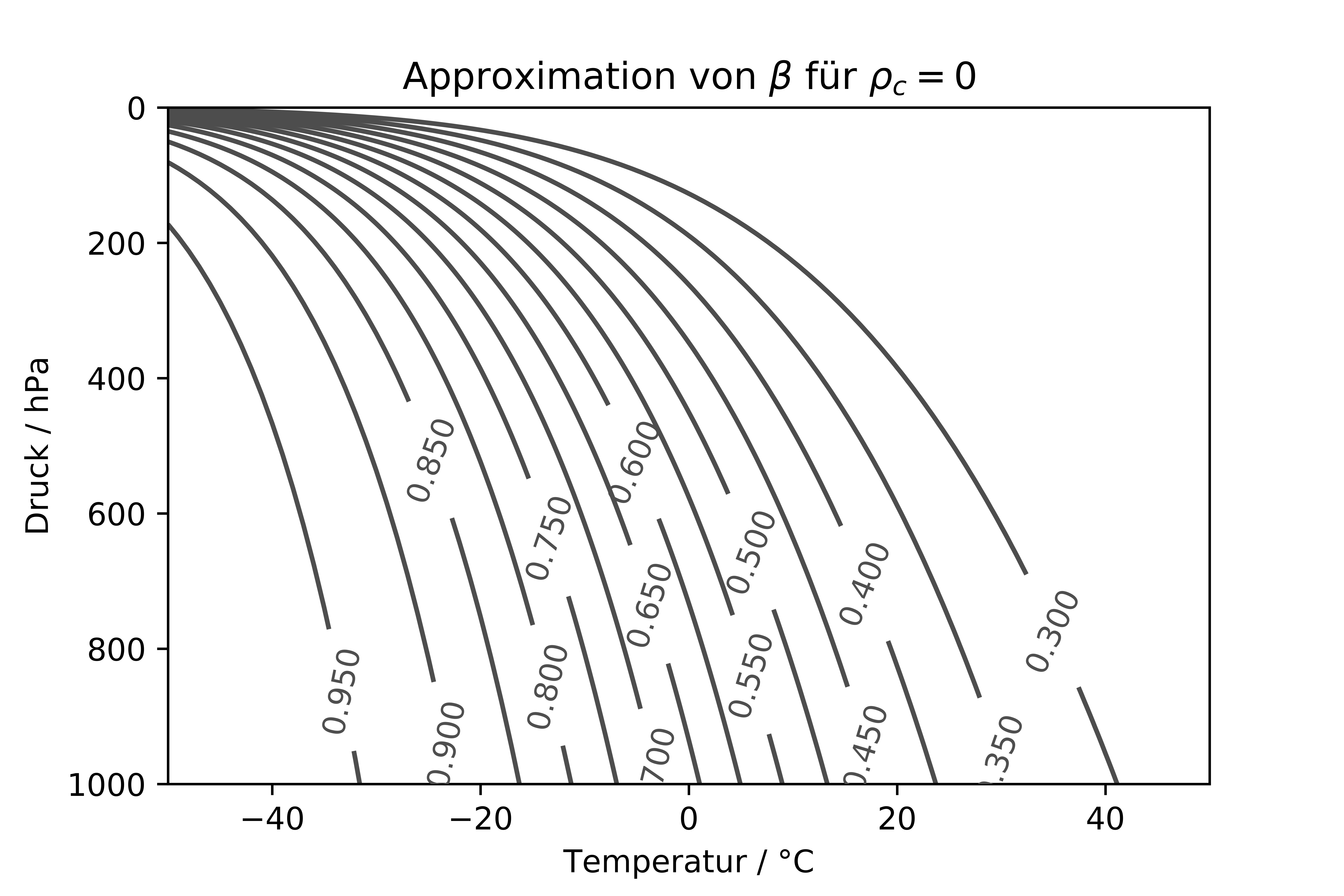
In the case of saturated air and

\[ \begin{align} \frac{\partial T}{\partial z} < -\Gamma_h \end{align} \]

the stratification is also unstable. In the case

\[ \begin{align} -\Gamma_d \leq \frac{\partial T}{\partial z} < -\Gamma_h \end{align} \]

the stratification is conditionally unstable, since only a saturated particle does not return to its rest position when deflected; the instability thus depends on the humidity. In the case of unsaturated air and

\[ \begin{align} \frac{\partial T}{\partial z} = -\Gamma_d \end{align} \]

or saturated air and

\[ \begin{align} \frac{\partial T}{\partial z} = -\Gamma_h \end{align} \]

one speaks of neutral stratification.

16.7.1.1 Equivalent potential temperature

To obtain the so-called equivalent potential temperature $\theta_e$ (also: pseudoequivalent potential temperature or, more rarely, pseudopotential temperature) of a particle, two steps are necessary:

1. Raise the particle dry adiabatically to its LCL.

2. Raise the particle irreversibly moist adiabatically to an infinite height. The potential temperature then obtained is $\theta_e$.

This quantity is thus adjusted not only for the pressure difference, but also for the existing moisture, which could lead to a temperature increase in the form of phase-transition enthalpy. It is therefore well suited to comparing the temperatures of different air masses.

16.7.1.2 Reversible equivalent potential temperature

The reversible equivalent potential temperature is defined analogously to the equivalent potential temperature, except that in step 2 of Sect. 16.7.1.1 a reversible wet adiabat is followed.

16.7.1.3 CAPE

The derivations in this section refer to a vertical air column and neglect dynamical effects caused by the velocity field. One defines a function $f\left(z, z'\right)$ as the specific force, i.e. the acceleration, acting on the particle at $z$ when it is brought adiabatically to the level $z'$ in a hydrostatic atmosphere:

\[ \begin{align} f\left(z, z'\right) \coloneqq -\frac{1}{\rho'\left(z, z'\right)}\frac{\partial p\left(z'\right)}{\partial z} - g \stackrel{\href{ch-12-important-approximations.html#eq:hydrostatic}{\text{Eq. (13.122)}}}{=} \frac{g\rho\left(z'\right)}{\rho'\left(z, z'\right)} - g = g\frac{\rho\left(z'\right) - \rho'\left(z, z'\right)}{\rho'\left(z, z'\right)}, \end{align} \]

where $\rho'\left(z, z'\right)$ is the density of the particle at $z$ after moving it adiabatically to $z'$. One also defines a function $\newtilde{F}\left(z, z'\right)$ by

\[ \begin{align} \newtilde{F}\left(z, z'\right) \coloneqq g\int_{z}^{z'}\frac{\rho\left(z''\right) - \rho'\left(z, z''\right)}{\rho'\left(z, z''\right)}dz'' \end{align} \]

as the work done by the stratification on a particle that was deflected adiabatically from $z$ to $z'$. Usually one chooses $z = z_{\mathrm{2m}} \coloneqq z_{\mathrm{SFC}} + 2$ m; one defines

\[ \begin{align} F\left(z\right) &\coloneqq \newtilde{F}\left(z_{\text{2m}}, z\right) = g\int_{z_{\text{2m}}}^{z}\frac{\rho\left(z''\right) - \rho'\left(z_{\text{2m}}, z''\right)}{\rho'\left(z_{\text{2m}}, z''\right)}dz'' = g\int_{z_{\text{2m}}}^{z}\frac{\rho\left(z'\right) - \rho'\left(z_{\text{2m}}, z'\right)}{\rho'\left(z_{\text{2m}}, z'\right)}dz'\nonumber\\ &= g\int_{z_{\text{2m}}}^{z}\frac{\rho\left(z'\right) - \rho'\left(z'\right)}{\rho'\left(z'\right)}dz' \end{align} \]

with the abuse of notation

\[ \begin{align} \rho'\left(z'\right) \coloneqq \rho'\left(z_{\text{2m}}, z'\right). \end{align} \]

For the integrand,

\[ \begin{align} f\left(z'\right) \coloneqq g\frac{\rho\left(z'\right) - \rho'\left(z'\right)}{\rho'\left(z'\right)}\tag{16.368}\label{eq:uplift} \end{align} \]

is likewise defined. Many of the quantities commonly used in connection with convection can be defined in terms of the functions $F$ and $f$. The so-called convectively available potential energy CAPE is defined by

\[ \begin{align} \CAPE \coloneqq \int_{z_{\text{2m}}}^{\infty}\Theta\left(f\left(z\right)\right)dz,\tag{16.369}\label{eq:def_cape} \end{align} \]

where $\Theta$ denotes the $\Theta $function. Realistically, of course, one does not integrate to infinity, but only up to a height $z_T$, where the tropopause is typically located, since above that there is no longer any instability anyway. In the case of dry air one can write for $f$

\[ \begin{align} f\left(z'\right) = g\frac{\frac{p}{R_dT} - \frac{p}{R_dT'}}{\frac{p}{R_dT'}} = g\frac{\frac{1}{T} - \frac{1}{T'}}{\frac{1}{T'}} = g\frac{T' - T}{T} = g\frac{\theta'\left(\frac{p}{p_0}\right)^{R_d/c_d^{(p)}} - \theta\left(\frac{p}{p_0}\right)^{R_d/c_d^{(p)}}}{\theta\left(\frac{p}{p_0}\right)^{R_d/c_d^{(p)}}} = g\frac{\theta' - \theta}{\theta}. \end{align} \]

In the case of moist air one can replace $T \to T_v$, where $T_v$ is the virtual temperature defined in Eq. (5.164), since at this temperature the dry air would have the same density as the existing moist air. The level of free convection $z_{\text{LFC}}$ is the height at which the adiabatically rising particle is for the first time lighter than the surroundings

\[ \begin{align} z_{\text{LFC}} \coloneqq\inf\{z\newvline f\left(z\right) > 0\}. \end{align} \]

When the particle reaches this height, it will continue to rise, which is called free convection, i.e. convection that would also take place without dynamic forcing. Analogously,

\[ \begin{align} z_{\text{EL}} \coloneqq\sup\{z\newvline f\left(z\right) > 0, z < 2z_T\} \end{align} \]

is called the equilibrium level. To be on the safe side, the deep stratosphere was excluded. This is the height at which a freely rising particle would be heavier than its surroundings. Often the $\Theta $function is omitted in Eq. (16.369) and one integrates only from $z_{\mathrm{LFC}}$ to $z_{\mathrm{EL}}$, which is correct precisely when thermal instability is present in exactly one height interval, as is often the case. The maximum cloud top is defined as the height at which such a particle would have lost its kinetic energy again, i.e

\[ \begin{align} z_{\text{MCT}} \coloneqq\inf\{z\newvline \newtilde{F}\left(z_{\text{LFC}}, z\right) < 0\}. \end{align} \]

The phenomenon $z_{\mathrm{MCT}} > z_{\mathrm{EL}}$ leads, in the case of deep convection, to the formation of gravity waves at the tropopause (overshooting tops), which is generally the case wherever a stably stratified height interval follows an unstably stratified one.

If a particle has reached the so-called trigger temperature at a height of two meters, it can rise into the LFC even without dynamic forcing, i.e.

\[ \begin{align} 0 \equiv g\int_{z_{\text{2m}}}^{z_{\text{LFC}}}\frac{\rho\left(z'\right) - \newtilde{\rho}'\left(z'\right)}{\newtilde{\rho}'\left(z'\right)}, \end{align} \]

where $\newtilde{\rho}'\left(z'\right)$ is the density of the particle lifted adiabatically from $z_{\mathrm{2m}}$ to $z'$, which would have the trigger temperature at a height of two meters. The energy $\CIN$ that must be overcome in the process, i.e.

\[ \begin{align} \CIN \coloneqq -\newtilde{F}\left(z_{\text{2m}}, z_{\text{LFC}}\right). \end{align} \]

is called the convective barrier or convective inhibition. The height at which a particle heated to the trigger temperature would be saturated during adiabatic ascent is called convective condensation level (CCL). This is at least as high as the LCL, so

\[ \begin{align} z_{\text{CCL}} \geq z_{\text{LCL}}. \end{align} \]

16.7.2 Kelvin-Helmholtz instability

The Kelvin-Helmholtz instability is the instability of a vertically sheared horizontal flow.

16.7.2.1 In discrete stratification

The motion is assumed to be y-symmetric, so the xz plane is considered. The xy plane coincides with the equilibrium position of a phase boundary. The medium above the boundary layer ($z > 0$) is given the index 1, the medium below it ($z < 0$) is given the index 2. The media are barotropic and incompressible. At time $t = 0$, the flow field is described by

\[ \begin{align} U_1 > 0, & {} & U_2 > 0, & {} & V_1 = V_2 = W_1 = W_2 = 0 \end{align} \]

The Coriolis force is neglected. One has

\[ \begin{align} \nabla \times \mathbf{v}_1 = \nabla \times \mathbf{v}_2 = \mathbf{0}. \end{align} \]

By the circulation theorem in the form Eq. (15.39), this also holds for $t > 0$ as long as the media do not mix. Therefore the velocity fields are described by two stream functions

\[ \begin{align} \psi_1 = U_1x + \psi_1', & {} & \psi_2 = U_2 x + \psi_2',\tag{16.379}\label{eq:khi_discrete_stream} \end{align} \]

where the primed quantities stand for the perturbations. Because of the absence of divergence,

\[ \begin{align} \Delta\psi_1' = \Delta\psi_2' = 0\tag{16.380}\label{eq:khi_deriv_laplace}. \end{align} \]

The deflection of the phase boundary is denoted by $\zeta$. With $\mathbf{n}$ as the normal vector of the surface and $\zeta$ as the surface deflection, the kinematic boundary condition holds

\[ \begin{align} \mathbf{n}\cdot\nabla\psi_1 = \mathbf{n}\cdot\left(\frac{\partial\zeta}{\partial t}\mathbf{e}_z\right) = \mathbf{n}\cdot\nabla\psi_2\text{ at }z = \zeta.\tag{16.381}\label{eq:khi_discrete_kbc} \end{align} \]

Neglecting the surface tension, the dynamic boundary condition follows

\[ \begin{align} p_1 = p_2\text{ at }z = \zeta.\tag{16.382}\label{eq:khi_discrete_dbc} \end{align} \]

For the normal vector $\mathbf{n}$, one has

\[ \begin{align} \mathbf{n} = \frac{1}{\sqrt{1 + \left(\frac{\partial\zeta}{\partial x}\right)^2}}\left(\begin{array}{c} -\frac{\partial\zeta}{\partial x}\\ 1\end{array}\right). \end{align} \]

The kinematic boundary condition Eq. (16.381) thus becomes

\[ \begin{align} -\left(U_1 + \frac{\partial\psi_1'}{\partial x}\right)\frac{\partial\zeta}{\partial x} + \frac{\partial\psi_1'}{\partial z} = \frac{\partial\zeta}{\partial t} = -\left(U_2 + \frac{\partial\psi_2'}{\partial x}\right)\frac{\partial\zeta}{\partial x} + \frac{\partial\psi_2'}{\partial z}\text{ at }z = \zeta, \end{align} \]

where the root expression was multiplied out. To linearize this expression, one applies it at $z = 0$ and neglects quadratic terms:

\[ \begin{align} -U_1\frac{\partial\zeta}{\partial x} + \frac{\partial\psi_1'}{\partial z} = \frac{\partial\zeta}{\partial t} = -U_2\frac{\partial\zeta}{\partial x} + \frac{\partial\psi_2'}{\partial z}\text{ at }z = 0\tag{16.385}\label{eq:khi_discrete_deriv_kbc} \end{align} \]

Since the flow field is irrotational and an ideal fluid is also assumed, one can use the time-dependent Bernoulli equations (see Eq. (15.122)) of the two layers

\[ \begin{align} \frac{\partial\psi_1}{\partial t} + \frac{1}{2}\left|\nabla\psi_1\right|^2 + \frac{p_1}{\rho_1} + gz &= C,\\ \frac{\partial\psi_2}{\partial t} + \frac{1}{2}\left|\nabla\psi_2\right|^2 + \frac{p_2}{\rho_2} + gz &= C_2 \end{align} \]

with real constants $C, C_2$. The dynamic boundary condition Eq. (16.382) implies the identity at $z = \zeta$

\[ \begin{align} \rho_1\left(C - \frac{\partial\psi_1}{\partial t} - \frac{1}{2}\left|\nabla\psi_1\right|^2 - gz\right) = \rho_2\left(C_2 - \frac{\partial\psi_2}{\partial t} - \frac{1}{2}\left|\nabla\psi_2\right|^2 - gz\right).\tag{16.388}\label{eq:khi_discrete_deriv_1} \end{align} \]

Without perturbation, one has

\[ \begin{align} \rho_1\left(C - \frac{1}{2}U_1^2\right) = \rho_2\left(C_2 - \frac{1}{2}U_2^2\right).\tag{16.389}\label{eq:khi_discrete_deriv_2} \end{align} \]

Subtracting Eq. (16.389) from Eq. (16.388) leads to

\[ \begin{align} \rho_1\left(-\frac{\partial\psi_1}{\partial t} + \frac{1}{2}U_1^2 - \frac{1}{2}\left|\nabla\psi_1\right|^2 - gz\right) = \rho_2\left(-\frac{\partial\psi_2}{\partial t} + \frac{1}{2}U_2^2 - \frac{1}{2}\left|\nabla\psi_2\right|^2 - gz\right),\tag{16.390}\label{eq:khi_discrete_deriv_3} \end{align} \]

which holds at $z = \zeta$. With Eqs. (16.379) - (16.379), it follows that

\[ \begin{align} \frac{1}{2}\left|\nabla\psi_j\right|^2 &= \frac{1}{2}\left(U_j^2 + \left(\frac{\partial\psi_j'}{\partial x}\right)^2 + 2U_j\frac{\partial\psi_j'}{\partial x} + \left(\frac{\partial\psi_j'}{\partial z}\right)^2\right) \end{align} \]

for $j = 1, 2$. Putting this into Eq. (16.390), one obtains

\[ \begin{align} & \rho_1\left(-\frac{\partial\psi_1}{\partial t} - \frac{1}{2}\left(\frac{\partial\psi_1'}{\partial x}\right)^2 - U_1\frac{\partial\psi_1'}{\partial x} - \frac{1}{2}\left(\frac{\partial\psi_1'}{\partial z}\right)^2 - gz\right)\nonumber\\ &= \rho_2\left(-\frac{\partial\psi_2}{\partial t} - \frac{1}{2}\left(\frac{\partial\psi_1'}{\partial x}\right)^2 - U_2\frac{\partial\psi_1'}{\partial x} - \frac{1}{2}\left(\frac{\partial\psi_1'}{\partial z}\right)^2 - gz\right),\tag{16.392}\label{eq:khi_discrete_deriv_4} \end{align} \]

at $z = \zeta.$ This equation is linearized by evaluating it at $z = 0$ and neglecting the quadratic terms:

\[ \begin{align} \rho_1\left(\frac{\partial\psi_1}{\partial t} + U_1\frac{\partial\psi_1'}{\partial x} + g\zeta\right) = \rho_2\left(\frac{\partial\psi_2}{\partial t} + U_2\frac{\partial\psi_1'}{\partial x} + g\zeta\right)\tag{16.393}\label{eq:khi_discrete_deriv_5} \end{align} \]

Now, for $j = 1, 2$, one makes the ansatz

\[ \begin{align} \psi_j' = A_j\left(z\right)\exp\left(ikx - i\omega t\right). \end{align} \]

With the Laplace equations Eq. (16.380), it follows that

\[ \begin{align} -k^2A_j + \frac{d^2A_j}{dz^2} &= 0. \end{align} \]

The solutions are of the form

\[ \begin{align} A_j\left(z\right) = A_\pm\exp\left(\pm kz\right). \end{align} \]

With the specifications

\[ \begin{align} \lim_{z \to\infty} \psi_1' = 0, & {} & \lim_{z \to -\infty} \psi_2' = 0, \end{align} \]

which mean that the perturbation should vanish at infinity, one obtains

\[ \begin{align} \psi_1' = A_-\exp\left[ikx - i\omega t - kz\right], & {} & \psi_2' = A_+\exp\left[ikx - i\omega t + kz\right]. \end{align} \]

For the surface deflection, one accordingly takes

\[ \begin{align} \zeta = \zeta_0\exp\left(ikx - i\omega t\right) \end{align} \]

Substituting this into Eqs. (16.385) and (16.393), one obtains

\[ \begin{align} -U_1ik\zeta_0 - kA_- &= -i\omega\zeta_0 = -U_2ik\zeta_0 + kA_+,\tag{16.400}\label{eq:khi_discrete_deriv_6}\\ \rho_1\left(-i\omega A_- + ikU_1A_- + g\zeta_0\right) &= \rho_2\left(-i\omega A_+ + ikU_2A_+ + g\zeta_0\right).\tag{16.401}\label{eq:khi_discrete_deriv_7} \end{align} \]

Eq. (16.400) implies

\[ \begin{align} A_- = \frac{i}{k}\zeta_0\left(\omega - U_1k\right), & {} & A_+ = \frac{i}{k}\zeta_0\left(U_2k - \omega\right). \end{align} \]

Putting this into Eq. (16.401), it follows that

\[ \begin{align} \rho_1\left(-i\omega\frac{i}{k}\zeta_0\left(\omega - U_1k\right) + ikU_1\frac{i}{k}\zeta_0\left(\omega - U_1k\right) + g\zeta_0\right) &= \rho_2\left(-i\omega\frac{i}{k}\zeta_0\left(U_2k - \omega\right) + ikU_2\frac{i}{k}\zeta_0\left(U_2k - \omega\right) + g\zeta_0\right)\nonumber\\ \Leftrightarrow\rho_1\left(\frac{\omega}{k}\left(\omega - U_1k\right) - U_1\left(\omega - U_1k\right) + g\right) &= \rho_2\left(\frac{\omega}{k}\left(U_2k - \omega\right) - U_2\left(U_2k - \omega\right) + g\right)\nonumber\\ \Leftrightarrow\rho_1\left(\omega\left(\omega - U_1k\right) - kU_1\left(\omega - U_1k\right) + kg\right) &= \rho_2\left(\omega\left(U_2k - \omega\right) - U_2k\left(U_2k - \omega\right) + kg\right). \end{align} \]

This is a quadratic equation for $\omega$, i.e. a dispersion relation. Further algebraic manipulation yields

\[ \begin{align} \omega^2 - 2k\omega\frac{\rho_1U_1 + \rho_2U_2}{\rho_1 + \rho_2} - kg\frac{\rho_2 - \rho_1}{\rho_1 + \rho_2} + k^2\frac{U_1^2\rho_1 + U_2^2\rho_2}{\rho_1 + \rho_2} = 0. \end{align} \]

This gives two solutions for the angular frequency:

\[ \begin{align} \omega_\pm &= \frac{\rho_1U_1k + \rho_2U_2k}{\rho_1 + \rho_2} \pm \left[kg\frac{\rho_2 - \rho_1}{\rho_1 + \rho_2} - k^2\frac{U_1^2\rho_1\rho_2 + U_2^2\rho_1\rho_2 - 2\rho_1\rho_2U_1U_2}{\left(\rho_1 + \rho_2\right)^2}\right]^{1/2}\nonumber\\ \Leftrightarrow\omega_\pm &= \frac{\rho_1U_1k + \rho_2U_2k}{\rho_1 + \rho_2} \pm \left[kg\frac{\rho_2 - \rho_1}{\rho_1 + \rho_2} - k^2\rho_1\rho_2\frac{\left(U_1 - U_2\right)^2}{\left(\rho_1 + \rho_2\right)^2}\right]^{1/2} \end{align} \]

Instability occurs in the case

\[ \begin{align} kg\frac{\rho_2 - \rho_1}{\rho_1 + \rho_2} &- k^2\rho_1\rho_2\frac{\left(U_1 - U_2\right)^2}{\left(\rho_1 + \rho_2\right)^2} < 0\nonumber\\ \Leftrightarrow kg\frac{\rho_2 - \rho_1}{\rho_1 + \rho_2} & < k^2\rho_1\rho_2\frac{\left(U_1 - U_2\right)^2}{\left(\rho_1 + \rho_2\right)^2}\nonumber \end{align} \]

so if

• the density difference is small enough,

• the wave is short enough or the

• speed difference is large enough.

An example is the formation of water surface waves under the influence of wind. One can assume that there are almost always spectral components in the wind field that satisfy the condition Eq. (16.406). The subsequent temporal development of the system can look different; for example, it depends on whether the media can mix or not.

16.7.2.2 In continuous stratification

One again considers the xz plane and neglects the Coriolis acceleration. One also makes the Boussinesq approximation (see Sect. 13.6). The momentum and continuity equations and the first law of thermodynamics read, with $\sigma$ as the potential density,

\[ \begin{align} \frac{\partial u}{\partial t} + u\frac{\partial u}{\partial x} + w\frac{\partial w}{\partial z} &= -\frac{1}{\rho}\frac{\partial p}{\partial x},\\ \frac{\partial w}{\partial t} + u\frac{\partial w}{\partial x} + w\frac{\partial w}{\partial z} &= -\frac{1}{\rho}\frac{\partial p}{\partial z} - g,\\ \frac{\partial u}{\partial x} + \frac{\partial w}{\partial z} &= 0,\\ \frac{\partial\sigma}{\partial t} + u\frac{\partial\sigma}{\partial x} + w\frac{\partial\sigma}{\partial z} &= 0. \end{align} \]

Now one assumes a vertically sheared background wind field $\newoverline{u}\left(z\right) = u\left(x, z, t\right) - u'\left(x, z, t\right)$, the vertical background wind $\newoverline{w}$ vanishes. The background density $\newoverline{\rho}\left(z\right) = \rho\left(x, z, t\right) - \rho'\left(x, z, t\right)$ is in hydrostatic balance with the background pressure field $\newoverline{p}\left(z\right) = p\left(x, z, t\right) - p'\left(x, z, t\right)$, i.e.

\[ \begin{align} \frac{\partial\newoverline{p}}{\partial z} &= -g\newoverline{\rho}.\tag{16.411}\label{eq:khi_deriv_1} \end{align} \]

Substituting this into the equations and linearizing them, one obtains

\[ \begin{align} \frac{\partial u'}{\partial t} + \newoverline{u}\frac{\partial u'}{\partial x} + w\frac{\partial\newoverline{u}}{\partial z} &= -\frac{1}{\rho}\frac{\partial p'}{\partial x} \approx -\frac{1}{\newtilde{\rho}}\frac{\partial p'}{\partial x},\\ \frac{\partial w}{\partial t} + \newoverline{u}\frac{\partial w}{\partial x} &= -\frac{1}{\rho}\frac{\partial p}{\partial z} - g \approx -\frac{1}{\newtilde{\rho}}\frac{\partial p}{\partial z} - \frac{g\rho}{\newtilde{\rho}} = -\frac{1}{\newtilde{\rho}}\frac{\partial p'}{\partial z} - \frac{g\rho'}{\newtilde{\rho}},\\ \frac{\partial u'}{\partial x} + \frac{\partial w}{\partial z} &= 0,\\ \frac{\partial\sigma'}{\partial t} + \newoverline{u}\frac{\partial\sigma'}{\partial x} + w\frac{\partial\newoverline{\sigma}}{\partial z} &= 0. \end{align} \]

In the x-component of the momentum equation, $\rho \to \newtilde{\rho}$ was replaced in the denominator of the pressure gradient term, where $\newtilde{\rho}$ denotes an average density assumed to be homogeneous; in the z-component, the right-hand side was multiplied by $\frac{\rho}{\newtilde{\rho}}$ before Eq. (16.411) was used. The perturbation of the flow is divergence-free, so one introduces a stream function $\psi = \psi\left(x, z, t\right)$ with

\[ \begin{align} u' = \frac{\partial\psi}{\partial z}, & {} &w = -\frac{\partial\psi}{\partial x} \end{align} \]

This means that the continuity equation is automatically satisfied. The remaining three equations read

\[ \begin{align} \frac{\partial^2\psi}{\partial t\partial z} + \newoverline{u}\frac{\partial^2\psi}{\partial z\partial x} - \frac{\partial\psi}{\partial x}\frac{\partial\newoverline{u}}{\partial z} &= -\frac{1}{\newtilde{\rho}}\frac{\partial p'}{\partial x},\\ -\frac{\partial^2\psi}{\partial t\partial x} - \newoverline{u}\frac{\partial^2\psi}{\partial x^2} &= -\frac{1}{\newtilde{\rho}}\frac{\partial p'}{\partial z} - \frac{g\rho'}{\newtilde{\rho}},\\ \frac{\partial\sigma'}{\partial t} + \newoverline{u}\frac{\partial\sigma'}{\partial x} - \frac{\partial\psi}{\partial x}\frac{\partial\newoverline{\sigma}}{\partial z} &= 0. \end{align} \]

One now further makes the ansätze

\[ \begin{align} \psi\left(x, z, t\right) = \psi_0\left(z\right)\exp\left[ik\left(x - ct\right)\right], & {} & p'\left(x, z, t\right) = p_0\left(z\right)\exp\left[ik\left(x - ct\right)\right],\\ \rho'\left(x, z, t\right) = \rho_0\left(z\right)\exp\left[ik\left(x - ct\right)\right], & {} & \sigma'\left(x, z, t\right) = \sigma_0\left(z\right)\exp\left[ik\left(x - ct\right)\right]. \end{align} \]

From this it follows

\[ \begin{align} -ikc\frac{d\psi_0}{dz} + \newoverline{u}ik\frac{d\psi_0}{dz} - ik\psi_0\frac{\partial\newoverline{u}}{\partial z} &= -ik\frac{p_0}{\newtilde{\rho}},\\ -k^2c\psi_0 + \newoverline{u}k^2\psi_0 &= -\frac{1}{\newtilde{\rho}}\frac{dp_0}{dz} -g\frac{\rho_0}{\newtilde{\rho}},\\ -ikc\sigma_0 + \newoverline{u}ik\sigma_0 -ik\psi_0\frac{d\newoverline{\sigma}}{dz} &= 0. \end{align} \]

Simplified, this gives

\[ \begin{align} -c\frac{d\psi_0}{dz} + \newoverline{u}\frac{d\psi_0}{dz} - \psi_0\frac{\partial\newoverline{u}}{\partial z} &= -\frac{p_0}{\newtilde{\rho}},\\ \psi_0k^2\left(\newoverline{u} - c\right) &= -\frac{1}{\newtilde{\rho}}\frac{dp_0}{dz} - g\frac{\rho_0}{\newtilde{\rho}}, \tag{16.426}\label{eq:khi_deriv_2}\\ \sigma_0\left(\newoverline{u} - c\right) - \psi_0\frac{d\newoverline{\sigma}}{dz} &= 0.\tag{16.427}\label{eq:khi_deriv_3} \end{align} \]

Differentiating the first equation with respect to $z$, one obtains

\[ \begin{align} \frac{d^2\psi_0}{dz^2}\left(\newoverline{u} - c\right) - \psi_0\frac{d^2\newoverline{u}}{dz^2} &= -\frac{1}{\newtilde{\rho}}\frac{dp_0}{dz}. \end{align} \]

Substituting Eq. (16.426) here, it follows that

\[ \begin{align} \left(\newoverline{u} - c\right)\left[\frac{d^2\psi_0}{dz^2} - k^2\psi_0\right] - \psi_0\frac{d^2\newoverline{u}}{dz^2} - g\frac{\rho_0}{\newtilde{\rho}} &= 0. \end{align} \]

To eliminate $\rho_0$, one first solves Eq. (16.427) for $\sigma_0$ and obtains

\[ \begin{align} \sigma_0 &= \frac{\psi_0}{\newoverline{u} - c}\frac{d\newoverline{\sigma}}{dz}. \end{align} \]

Without loss of generality, one can place the reference level at the level currently under consideration and use $\rho_0 = \sigma_0$. Substituting this gives

\[ \begin{align} \left(\newoverline{u} - c\right)\left[\frac{d^2\psi_0}{dz^2} - k^2\psi_0\right] -\psi_0\frac{d^2\newoverline{u}}{dz^2} - \frac{\psi_0}{\newoverline{u} - c}\frac{g}{\newtilde{\rho}}\frac{d\newoverline{\sigma}}{dz} &= 0. \end{align} \]

Here one inserts the Brunt-Väisälä frequency

\[ \begin{align} N^2 \coloneqq -\frac{g}{\newtilde{\rho}}\frac{d\newoverline{\sigma}}{dz} \end{align} \]

and obtains

\[ \begin{align} \left(\newoverline{u} - c\right)\left(\frac{d^2}{dz^2} - k^2\right)\psi + \left(\frac{N^2}{\newoverline{u} - c} - \frac{d^2\newoverline{u}}{dz^2}\right)\psi = 0.\tag{16.433}\label{eq:taylor-goldstein} \end{align} \]

This equation is called the Taylor-Goldstein equation. It is an eigenvalue problem $\left\{\psi, c\right\}$ for the function $\psi$ with the eigenvalue $c$ depending on $\newoverline{u}\left(z\right)$. If $\left\{\psi, c\right\}$ is a solution, then $\left\{\psi^\star, c^\star\right\}$ is also a solution. A positive imaginary part of $c$ means that $\psi$ is an unstable solution. A shear $\newoverline{u} = \newoverline{u}\left(z\right)$ is stable if and only if all solutions of Eq. (16.433) have real eigenvalues. It is now further assumed that at $z = 0, H$ the boundary conditions $w = 0$ hold, from which it follows

\[ \begin{align} \psi\left(0\right) = \psi\left(H\right) = 0. \end{align} \]

Now one defines $\phi$ by

\[ \begin{align} \psi = \sqrt{\newoverline{u} - c}\phi. \end{align} \]

Differentiating with respect to $z$ gives

\[ \begin{align} \frac{d\psi}{dz} &= \frac{1}{2}\frac{1}{\sqrt{\newoverline{u} - c}}\phi\frac{d\newoverline{u}}{dz} + \sqrt{\newoverline{u} - c}\frac{d\phi}{dz},\\ \Rightarrow\frac{d^2\psi}{dz^2} &= \frac{1}{\sqrt{\newoverline{u} - c}}\frac{d\newoverline{u}}{dz}\frac{d\phi}{dz} - \frac{1}{4}\frac{1}{\sqrt{\newoverline{u} - c}^3}\phi\left(\frac{d\newoverline{u}}{dz}\right)^2 + \frac{1}{2}\frac{1}{\sqrt{\newoverline{u} - c}}\frac{d^2\newoverline{u}}{dz^2}\phi + \sqrt{\newoverline{u} - c}\frac{d^2\phi}{dz^2}. \end{align} \]

Putting this into Eq. (16.433) and dividing by $\sqrt{\newoverline{u} - c}$, one obtains

\[ \begin{align} \frac{d}{dz}\left[\left(\newoverline{u} - c\right)\frac{d\phi}{dz}\right] - \left[k^2\left(\newoverline{u} - c\right) + \frac{1}{2}\frac{d^2\newoverline{u}}{dz^2} + \frac{1}{\newoverline{u} - c}\left(\frac{1}{4}\left(\frac{d\newoverline{u}}{dz}\right)^2 - N^2\right)\right]\phi = 0.\tag{16.438}\label{eq:khi_deriv_4} \end{align} \]

Under the assumption $c \not= \newoverline{u}$, the boundary conditions remain

\[ \begin{align} \phi\left(0\right) = \phi\left(H\right) = 0. \end{align} \]

Eq. (16.438) is now multiplied by $\phi^\star$:

\[ \begin{align} \phi^\star\frac{d}{dz}\left[\left(\newoverline{u} - c\right)\frac{d\phi}{dz}\right] - \left[k^2\left(\newoverline{u} - c\right) + \frac{1}{2}\frac{d^2\newoverline{u}}{dz^2} + \frac{1}{\newoverline{u} - c}\left(\frac{1}{4}\left(\frac{d\newoverline{u}}{dz}\right)^2 - N^2\right)\right]\left|\phi\right|^2 = 0.\tag{16.440}\label{eq:khi_deriv_5} \end{align} \]

Integrating the first term from $0$ to $H$, it follows by integration by parts

\[ \begin{align} \int_0^H\phi^\star\frac{d}{dz}\left[\left(\newoverline{u} - c\right)\frac{d\phi}{dz}\right]dz &= -\int_0^H\left(\newoverline{u} - c\right)\left|\frac{d\phi}{dz}\right|^2dz. \end{align} \]

Eq. (16.440) is now integrated from $0$ to $H$:

\[ \begin{align} \int_0^H\left[N^2 - \frac{1}{4}\left(\frac{d\newoverline{u}}{dz}\right)^2\right]\frac{\left|\phi\right|^2}{\newoverline{u} - c}dz &= \int_0^H\left(\newoverline{u} - c\right)\left(\left|\frac{d\phi}{dz}\right|^2 + k^2\left|\phi\right|^2\right) + \frac{1}{2}\frac{d^2\newoverline{u}}{dz^2}\left|\phi\right|^2dz.\tag{16.442}\label{eq:khi_deriv_6} \end{align} \]

Now one writes for the phase velocity

\[ \begin{align} c = c_r + ic_i \end{align} \]

with $c_r, c_i\in \mathbb{R}$. The imaginary part of Eq. (16.442) reads

\[ \begin{align} c_i\int_0^H\left[N^2 - \frac{1}{4}\left(\frac{d\newoverline{u}}{dz^2}\right)^2\right]\frac{\left|\phi\right|^2}{\left|\newoverline{u} - c\right|^2}dz &= -c_i\int_0^H\left(\left|\frac{d\phi}{dz}\right|^2 + k^2\left|\phi\right|^2\right)dz\nonumber\\ \Rightarrow c_i\int_0^H\left[N^2 - \frac{1}{4}\left(\frac{d\newoverline{u}}{dz^2}\right)^2\right]\frac{\left|\phi\right|^2}{\left|\newoverline{u} - c\right|^2} + \left|\frac{d\phi}{dz}\right|^2 + k^2\left|\phi\right|^2dz &= 0. \end{align} \]

If $N^2 - \frac{1}{4}\left(\frac{d\newoverline{u}}{dz^2}\right)^2 > 0$ everywhere in the interval $\left(0, H\right), $ then $c_i = 0$. One defines the Richardson number $R_i$ by

The frequency

is called Prandtl frequency. The condition

is sufficient for stability.

16.7.3 Barotropic instability

Assume a westerly base current $U>0$ that depends only on $y$

\[ \begin{align} U = U\left(y\right) \end{align} \]

and a perturbation

\[ \begin{align} \mathbf{v}_h' = \left(u, v\right)^T = \mathbf{k}\times\nabla\psi \end{align} \]

with a stream function $\psi$. Consider a zonal channel of extent $2b$ with $b>0$, the line $y = 0$ lies in the middle of this channel. The boundary conditions are $\omega = 0$ at $p = 0$ and $p = p_0$ and $v = 0$ at $y = \pm b$. Then the horizontal wind is divergence-free and the barotropic vorticity equation can be applied,

\[ \begin{align} \frac{\partial\zeta}{\partial t} + \beta v + u\frac{\partial\zeta}{\partial x} + v\frac{\partial\zeta}{\partial y} = 0. \end{align} \]

Here $\beta$ is homogeneous, see Sect. 13.9.2. Making a perturbation ansatz according to Sect. 16.3, one obtains

\[ \begin{align} \frac{\partial\zeta'}{\partial t} + \beta v + U\frac{\partial\zeta'}{\partial x} + v\frac{\partial\newoverline{\zeta}}{\partial y} = 0. \end{align} \]

Here the vorticity was written $\zeta = \newoverline{\zeta} + \zeta'$ with $\newoverline{\zeta}$ as the vorticity of $U$ and $\zeta'$ as the vorticity of $\mathbf{v}_h'$. For the perturbation, one sets

\[ \begin{align} \psi\left(x, y, t\right) = Y\left(y\right)\psi_0e^{i\left(kx - \omega t\right)} \end{align} \]

With $Y\left(\pm b\right)\hastobe0$ the boundary conditions on $v$ are satisfied, one also obtains

\[ \begin{align} v &= \frac{\partial\psi}{\partial x} = ik\psi,\\ \zeta' &= \Delta \psi = -k^2\psi + Y''\psi_0e^{i(kx - \omega t)},\\ \frac{\partial\zeta'}{\partial x} &= -ik^3\psi + Y''\psi_0ike^{i\left(kx - \omega t\right)}.\\ \end{align} \]

Plugging this into the barotropic vorticity equation and cancelling $\psi_0e^{i\left(kx - \omega t\right)}$, one obtains

\[ \begin{align} i\omega k^2Y - i\omega Y'' + \beta ikY - Uik^3Y + Y''ikU - ikY\frac{d^2U}{dy^2} &= 0\nonumber\\ \Leftrightarrow \omega k^2Y - \omega Y'' + \beta kY - Uk^3Y + Y''kU - kY\frac{d^2U}{dy^2} &= 0\tag{16.457}\label{eq:baro_inst_deriv_1}. \end{align} \]

Instability means that $\omega$ is not purely real,

\[ \begin{align} \omega = \omega_r + i\omega _c, \end{align} \]

with $\omega_r, \omega_c\in \mathbb{R}\setminus\{0\}$. Substituting into Eq. (16.457) gives

\[ \begin{align} k^2Y\left(\omega_r + i\omega_c\right) - Y''\left(\omega_r + i\omega_c\right) + \beta kY - Uk^3Y + Y''kU = 0. \end{align} \]

The imaginary part of this is

\[ \begin{align} k^2Y\omega_c - Y''\omega_c = 0\Leftrightarrow Y'' = k^2Y. \end{align} \]

Substituting this into the real part, one obtains

\[ \begin{align} k^2Y\omega_r& - k^2Y\omega_r + \beta kY - Uk^3Y + Uk^3Y - kY\frac{d^2U}{dy^2} = 0\Rightarrow\frac{d^2U}{dy^2} = \beta.\tag{16.461}\label{eq:notw_baro_inst} \end{align} \]

This is a necessary condition. Conversely, assuming Eq. (16.461), Eq. (16.457) becomes (one does not yet know here whether $\omega$ is real)

\[ \begin{align} \omega k^2Y - \omega Y'' - Uk^3Y + Y''kU = 0.\tag{16.462}\label{eq:baro_inst_deriv_2} \end{align} \]

Assuming a jet-shaped background wind

\[ \begin{align} U\left(y\right) = U_{\text{min}} + \frac{1}{2}\left(U_{\text{max}} - U_{\text{min}}\right)\left(1 + e^{i \frac{y\pi}{b}}\right) \end{align} \]

with $U_{\mathrm{min}}, U_{\mathrm{max}}>0$, one obtains in the imaginary part of Eq. (16.462)

\[ \begin{align} k^3Y\frac{1}{2}\left(U_{\text{max}} - U_{\text{min}}\right)\sin\left(\frac{y\pi}{b}\right) = Y''k\frac{1}{2}\left(U_{\text{max}} - U_{\text{min}}\right)\sin\left(\frac{y\pi}{b}\right), \end{align} \]

hence

\[ \begin{align} Y'' = k^2Y. \end{align} \]

The fact that a state is unstable does not necessarily mean that it will collapse. However, an arbitrarily small initial deflection $v$ is sufficient to generate an exponentially growing perturbation. In reality one can assume the existence of such a very small initial perturbation, so that instability in reality always leads to the collapse of the basic state.

16.7.4 Baroclinic instability

For the expression under the square root in Eq. (16.311), an abbreviation

\[ \begin{align} g = g\left(\newoverline{u}_T, k\right) \coloneqq\frac{\beta^2K^4}{4k^2} + \newoverline{u}_T^2k^2\left(k^4 - K^4\right) \end{align} \]

is now defined. In the case $g<0$, one has

\[ \begin{align} \omega = \omega_r + i\frac{1}{k^2 + K^2}\omega_i' \end{align} \]

with

\[ \begin{align} \omega_i' \coloneqq\pm\sqrt{\left|g\left(\newoverline{u}_T, k\right)\right|}. \end{align} \]

This means that in the case of the negative sign the amplitude grows exponentially, so an instability is present. Define

\[ \begin{align} N \coloneqq\frac{\omega_i'}{k^2 + K^2} = \frac{\sqrt{\left|g\left(\newoverline{u}_T, k\right)\right|}}{k^2 + K^2}, \end{align} \]

this is the growth constant of the perturbation. In the unstable case, one thus has

\[ \begin{align} N^2 + \frac{g}{\left(k^2 + K^2\right)} &= N^2 + \frac{\frac{\beta^2K^4}{4k^2} + \newoverline{u}_T^2k^2\left(k^4 - K^4\right)}{\left(k^2 + K^2\right)^2} = 0. \end{align} \]

At this point one defines a dimensionless angular wavenumber

\[ \begin{align} \kappa \coloneqq\frac{k}{K}, \end{align} \]

it then follows that

\[ \begin{align} N^2 + \frac{\frac{\beta^2}{4k^2} + \newoverline{u}_T^2k^2\left(\kappa^2 + 1\right)\left(\kappa^2 - 1\right)}{\left(\kappa^2 + 1\right)^2} &= N^2 + \frac{\beta^2}{4k^2\left(\kappa^2 + 1\right)^2} + \newoverline{u}_T^2k^2\frac{\kappa^2 - 1}{\kappa^2 + 1} = 0\nonumber\\ \Rightarrow N^2 + \frac{\beta^2}{4k^2\left(\kappa^2 + 1\right)^2} + \frac{\beta^2}{K^2}\newoverline{u}^{\star2}_T\kappa^2\frac{\kappa^2 - 1}{\kappa^2 + 1} &= 0 \end{align} \]

with a dimensionless thermal wind

\[ \begin{align} \newoverline{u}_T^\star \coloneqq\frac{\newoverline{u}_TK^2}{\beta}. \end{align} \]

From this it follows

\[ \begin{align} \frac{N^2K^2}{\kappa^2\beta^2} + \frac{1}{4\kappa^4\left(\kappa^2 + 1\right)^2} + \newoverline{u}^{\star2}_T\frac{\kappa^2 - 1}{\kappa^2 + 1} &= 0 \end{align} \]

With the dimensionless growth rate

\[ \begin{align} n \coloneqq\frac{NK}{\kappa\beta} \end{align} \]

one can write this as

\[ \begin{align} n^2 + \frac{1}{4\kappa^4\left(\kappa^2 + 1\right)^2} + \newoverline{u}^{\star2}_T\frac{\kappa^2 - 1}{\kappa^2 + 1} &= 0 \end{align} \]

Solving this for $\newoverline{u}^{\star2}_T$, it follows that

\[ \begin{align} \newoverline{u}^{\star2}_T = n^2\frac{1 + \kappa^2}{1 - \kappa^2} + \frac{1}{4\kappa^4\left(1 - \kappa^4\right)}. \end{align} \]

Fig. 16.7 shows the thermal wind shear required for different wave numbers and growth rates. From the definitions of $\kappa$ and $\newoverline{u}^\star_T$ it is clear that as thermal stability decreases, one moves to the top left in this representation, i.e. towards baroclinic instability.

In baroclinic instability, potential energy of the stratification, which is continually generated by the radiation field, is converted into kinetic energy of the horizontal wind before it is dissipated.