17 turbulence

There is no mathematically exact definition of whether a flow field is turbulent or not. It can be assumed that any flow field, if viewed from a sufficiently large distance, will appear tubulent. However, if you zoom in far enough, you will usually find a scale on which the field makes a laminar impression, which is understood as the opposite of turbulence. If this scale is the molecular scale, full turbulence is present.

17.1 Basics

Define an averaging operator by

\[ \begin{align} \newoverline{f} \coloneqq \frac{1}{\mu\left(\Omega\right)}\int_\Omega fd\omega,\tag{17.1}\label{eq:simple_average} \end{align} \]

where $\Omega$ should be an arbitrary spatial and/or temporal quantity, $\mu\left(\Omega\right)$ its measure, $f$ an arbitrary function of space and time and $d\omega$ a suitable differential. Now you can use $f$ in the form

\[ \begin{align} f & \equiv \newoverline{f} + f' \end{align} \]

dismantle; For this purpose, the fluctuation or turbulence is defined by

\[ \begin{align} f' &\coloneqq f - \newoverline{f}. \end{align} \]

If the statements

\[ \begin{align} \newoverline{\frac{\partial f}{\partial x_i}} &= \frac{\partial\newoverline{f}}{\partial x_i}, \tag{17.4}\label{eq:reynolds_prop_1}\\ \newoverline{\frac{\partial f}{\partial t}} &= \frac{\partial\newoverline{f}}{\partial t}, \tag{17.5}\label{eq:reynolds_prop_2}\\ \newoverline{f'\newoverline{g}} &= 0\tag{17.6}\label{eq:reynolds_prop_3} \end{align} \]

with an arbitrary field $g$, $\newoverline{f}$ is called Reynolds operator and the corresponding averaging is called Reynolds averaging. It is easy to realize that this also results in the two statements

\[ \begin{align} \newoverline{f'} = 0, & {} & \newoverline{\newoverline{f}} = \newoverline{f} \end{align} \]

consequences. At this point we don't care about what such an operator could actually look like; in Section 17.1.2 it will be stated that the usual averaging operators are not Reynolds operators. From now on, however, Eq. (17.1) is used, instead the Hesselberg mean

\[ \begin{align} \left\langle f\right\rangle \coloneqq \frac{1}{\int_\Omega\rho d\omega}\int_\Omega\rho fd\omega\tag{17.8}\label{eq:hesselberg-average} \end{align} \]

used, where $\rho$ is the density. You now write for the fluctuation

\[ \begin{align} f'' \coloneqq f - \left\langle f\right\rangle. \end{align} \]

It is now assumed that the Hesselberg mean is a Reynolds operator. Applying this to the dry adiabatic system of equations follows

\[ \begin{align} \frac{\partial\newoverline{\mathbf{v}}}{\partial t} &= -\left(\newoverline{\mathbf{v}}\cdot\nabla\right)\newoverline{\mathbf{v}} - \newoverline{\left(\mathbf{v}''\cdot\nabla\right)\mathbf{v}''} - \newoverline{\alpha}\frac{\partial\newoverline{p}}{\partial x} - \newoverline{\alpha''\frac{\partial p'}{\partial x}} - \mathbf{f}\times\newoverline{\mathbf{v}} + \mathbf{g},\\ \frac{\partial\newoverline{\theta}}{\partial t}&= -\newoverline{\mathbf{v}}\cdot\nabla\newoverline{\theta} - \newoverline{\mathbf{v}''\cdot\nabla\theta''} ,\\ \frac{\partial\newoverline{\rho}}{\partial t} &= -\newoverline{\rho}\nabla\cdot\newoverline{\mathbf{v}} - \newoverline{\mathbf{v}}\cdot\nabla\newoverline{\rho} - \newoverline{\rho''\nabla\cdot\mathbf{v}''} - \newoverline{\mathbf{v}''\cdot\nabla\rho''},\\ \newoverline{p}\newoverline{\alpha}&= R_d\newoverline{T} - \newoverline{p''\alpha''}. \end{align} \]

The prognostic equations of the averaged fields are therefore corrected compared to those of the unaveraged fields by terms of the form $\newoverline{f''g''}$, where $f, g$ are linear in the fields and their derivatives. These terms are referred to as the convergences of the turbulent correlation flow. These of course depend on the size of the quantity being averaged over, i.e. h. in the case of a numerical model, it depends on the resolution. As the averaging amount becomes smaller and smaller, the covariance terms become less important until they finally disappear completely.

However, there are no prognostic equations for the turbulent quantities, which is referred to as the closure problem. To further specify the correlation terms in the momentum equation, one applies the Reynolds averaging operator to Eq. (8.15), you get like this

\[ \begin{align} \frac{\partial\left(\rho\mathbf{v}\right)}{\partial t} + \nabla p + \nabla\cdot\Pi - \rho\mathbf{g} + \nabla\cdot\newtilde{\Pi} = \mathbf{0}, \end{align} \]

where the horizontal lines have been omitted for clarity. Furthermore, the turbulence correlation tensor $\newtilde{\Pi}$ is through

\[ \begin{align} \newtilde{\Pi} \coloneqq \rho\left(\begin{array}{ccc} \newoverline{u''u''} & \newoverline{u''v''} & \newoverline{u''w''} \\ \newoverline{v''u''} & \newoverline{v''v''} & \newoverline{v''w''} \\ \newoverline{w''u''} & \newoverline{w''v''} & \newoverline{w''w''} \end{array}\right) =: \left(\begin{array}{ccc} \newtilde{\Pi}_{x, x} & \newtilde{\Pi}_{x, y} & \newtilde{\Pi}_{x, z} \\ \newtilde{\Pi}_{y, x} & \newtilde{\Pi}_{y, y} & \newtilde{\Pi}_{y, z} \\ \newtilde{\Pi}_{z, x} & \newtilde{\Pi}_{z, y} & \newtilde{\Pi}_{z, z} \end{array}\right) \end{align} \]

defined. It was justified by the assumption

\[ \begin{align} \left|\frac{\rho''}{\newoverline{\rho}}\right| \ll \left|\frac{u''}{\newoverline{u}}\right| \end{align} \]

went out. $-\nabla\cdot\newtilde{\Pi}$ provides the Eddy stress terms, which are reflected in the momentum equation and instead of the $- \newoverline{\left(\mathbf{v}''\cdot\nabla\right)\mathbf{v}''} - \newoverline{\alpha''\frac{\partial p''}{\partial x}}$ can be used.

17.1.1 Turbulent dissipation

Analogous to the molecular dissipation $\epsilon$ (see equation (8.66)), one can have a turbulent dissipation associated with the turbulence

define. Since there is no explicit formula for $\newtilde{\Pi}$, one cannot find a turbulent analogue to Eq. Find (8.90): The sign of $\epsilon_\text{turb}$ remains undetermined.

17.1.2 Concrete averaging operators

Let $f$ be a scalar or vector function of position and time. A general averaging operator $\newoverline{f}$ is defined by

\[ \begin{align} \newoverline{f}\left(x_i\right) \coloneqq \frac{\int_\Omega f\left(x_i\right)h\left(x_i\right)dx_1\dotsc dx_n}{\int_\Omega h\left(x_i\right)dx_1\dotsc dx_n}, \tag{17.18}\label{eq:av_op_gen} \end{align} \]

where the time $t$ should be understood as one of the $x_i$ and $h$ represents a weighting function.

17.1.2.1 Moving time average

The moving time average with the averaging length $T$ is obtained from Eq. (17.18) with $\Omega = \left(t - \frac{T}{2}, t + \frac{T}{2}\right)$ and $h = 1$, so

\[ \begin{align} \newoverline{f}\left(\mathbf{r}, t\right) = \frac{1}{T}\int_{t-\frac{T}{2}}^{t + \frac{T}{2}}f\left(\mathbf{r}, t'\right)dt'. \end{align} \]

One now checks whether this operator fulfills the properties of a Reynolds operator equations (17.4) - (17.6). First of all

\[ \begin{align} \frac{\partial\overline{f}}{\partial x_i} &= \frac{1}{T}\int_{t-\frac{T}{2}}^{t + \frac{T}{2}}\frac{\partial f}{\partial x_i}\left(\mathbf{r}, t'\right)dt' = \newoverline{\frac{\partial f}{\partial x_i}}, \end{align} \]

Eq. (17.4) is therefore fulfilled. The verification of the fulfillment of Eq. (17.5) is done using the main theorem of differential and integral calculus:

\[ \begin{align} \frac{\partial\overline{f}}{\partial t} &= \frac{f\left(\mathbf{r}, t + \frac{T}{2}\right) - f\left(\mathbf{r}, t - \frac{T}{2}\right)}{T} = \frac{1}{T}\int_{t-\frac{T}{2}}^{t + \frac{T}{2}}\frac{\partial f}{\partial t'}\left(\mathbf{r}, t'\right)dt' = \newoverline{\frac{\partial f}{\partial t}} \end{align} \]

The first two properties are therefore fulfilled. For the third one calculates with $g = 1$

\[ \begin{align} \newoverline{f'} &= \frac{1}{T}\int_{t-\frac{T}{2}}^{t + \frac{T}{2}}f\left(\mathbf{r}, t'\right) - \newoverline{f}\left(\mathbf{r}, t'\right)dt' \hastobe 0. \end{align} \]

This should apply to any point in time, so it follows from this

\[ \begin{align} \newoverline{f} = f \end{align} \]

at all times as a criterion for the validity of Eq. (17.6) for the simple case $g = 1$, which is only the case for linear functions $f$.

17.1.2.2 Hesselberg means

If you put in Eq. (17.18) the case $h = \rho$, one obtains the Hesselberg mean already mentioned in the introduction. For this you note the decomposition

\[ \begin{align} f = \left\langle f\right\rangle + f'', \end{align} \]

to use the Hesselberg mean from other averages such as B. the moving time average or a general Reynolds operator.

17.1.2.3 Low pass

The Fourier transform $\newtilde{f}\left(k\right)$ of a field $f = f\left(x\right)$ is

\[ \begin{align} \newtilde{f}\left(k\right) \stackrel{\href{ch-41-orthogonal-function-systems.html#eq:def_ft_1d}{\text{Glg. (C.3)}}}{=} C\int_{-\infty}^\infty f\left(x\right)\exp\left(-ikx\right)dx. \end{align} \]

The inverse Fourier transformation is according to Eq. (C.6) given by

\[ \begin{align} f\left(x\right) = \newtilde{C}\int_{-\infty}^\infty f\left(x\right)\exp\left(ikx\right)dk, \end{align} \]

where according to Eq. (C.9) pay attention to $C\newtilde{C} = 1/\left(2\pi\right)$. A low pass with the cutoff wave number $k^\star > 0$ is given by the equation

\[ \begin{align} \newoverline{f}\left(x\right) = \newtilde{C}\int_{-k^\star}^{k^\star}f\left(x\right)\exp\left(ikx\right)dk \end{align} \]

set. As already indicated by the notation $\newoverline{f}$, this is also a type of averaging operator. For the fluctuation $f'$ one obtains

\[ \begin{align} f'\left(x\right) &\coloneqq f\left(x\right) - \newoverline{f}\left(x\right) = \newtilde{C}\int_{-\infty}^{\infty}f\left(x\right)\exp\left(ikx\right)dk - \newtilde{C}\int_{-k^\star}^{k^\star}f\left(x\right)\exp\left(ikx\right)dk\nonumber\\ &= \newtilde{C}\int_{-\infty}^{-k^\star}f\left(x\right)\exp\left(ikx\right)dk + \newtilde{C}\int_{k^\star}^{\infty}f\left(x\right)\exp\left(ikx\right)dk. \end{align} \]

17.2 Mixing path approach

However, the $\tau_{i, j}$ are still unknown quantities. In order to parameterize them (see also section 17.9), one uses the mixing path approach. It is assumed that the pressure gradient and Coriolis force do not play a significant role, which is why

\[ \begin{align} \md{\mathbf{v}} = \mathbf{0}\tag{17.29}\label{eq:burgers_eq} \end{align} \]

follows what is called Burgers equation. Accordingly, every fluid particle moves along a straight, uniform path. However, this is not a completely sensible approach, but it does provide a useful way to parameterize the $u'', v'', w''$. If a particle moves from $z$ to $z + l$ while maintaining its horizontal velocity $\mathbf{v}_h$, Eq. (17.29)

\[ \begin{align} \mathbf{v}_h''\left(z + l\right) = \mathbf{v}_h\left(z + l\right) - \overline{\mathbf{v}_h}\left(z + l\right) = \newoverline{\mathbf{v}_h}\left(z\right) - \overline{\mathbf{v}_h}\left(z + l\right) = \overline{\mathbf{v}_h}\left(z + l\right) - l\frac{\partial\newoverline{\mathbf{v}_h}}{\partial z} - \overline{\mathbf{v}_h}\left(z + l\right) = -l\frac{\partial\newoverline{\mathbf{v}_h}}{\partial z} \end{align} \]

Please also note the sign of $l$, which must be understood as negative in the case of downward movement. This follows, for example:

\[ \begin{align} \tau_{x, z} = -\rho\newoverline{u''w''} = \rho\newoverline{w''l}\frac{\partial\newoverline{u}}{\partial z}. \end{align} \]

In the case of an indifferently layered atmosphere, $\left|w''\right| applies \sim \left|\mathbf{v}_h''\right|$, which corresponds to the fact that in this case the horizontal scale of the vortices is the same size as the vertical one, one therefore sets

\[ \begin{align} w'' = l\left|\frac{\partial\overline{\mathbf{v}_h}}{\partial z}\right|. \end{align} \]

It follows

\[ \begin{align} \tau_{x, z} = -\rho\newoverline{u'w'} = \rho\newoverline{l^2}\left|\frac{\partial\newoverline{\mathbf{v}_h}}{\partial z}\right|\frac{\partial\newoverline{u}}{\partial z} \equiv A_z\frac{\partial\overline{u}}{\partial z}.\tag{17.33}\label{eq:eddy_corr_para} \end{align} \]

The coefficient

\[ \begin{align} A_z \coloneqq \rho\newoverline{l^2}\left|\frac{\partial\newoverline{\mathbf{v}_h}}{\partial z}\right|\tag{17.34}\label{eq:def_eddy_exchange_coeff} \end{align} \]

is called Eddy exchange coefficient.

17.2.1 Planetary boundary layer

The planetary boundary layer is defined as the lower layer of the atmosphere in which the ground friction, i.e. h. the existence of the earth's surface has an influence. This is where the balance of power comes in

\[ \begin{align} -fv &= -\frac{1}{\rho}\frac{\partial p}{\partial x} + \frac{1}{\rho}\frac{\partial\tau_{x, z}}{\partial z}, \tag{17.35}\label{eq:friction_boundary_equilibrium_x}\\ fu &= -\frac{1}{\rho}\frac{\partial p}{\partial y} + \frac{1}{\rho}\frac{\partial\tau_{y, z}}{\partial z}.\tag{17.36}\label{eq:friction_boundary_equilibrium_y} \end{align} \]

where the averaging operators have been omitted again for the sake of clarity. The horizontal correlation flows were also omitted at this point. If one also assumes that the density varies only slightly within the altitude interval under consideration, it follows

\[ \begin{align} -fv &= -\frac{1}{\rho}\frac{\partial p}{\partial x} + \frac{\partial}{\partial z}\left(\frac{\tau_{x, z}}{\rho}\right), \tag{17.37}\label{eq:momentum_tau_z_ind_x}\\ fu &= -\frac{1}{\rho}\frac{\partial p}{\partial y} + \frac{\partial}{\partial z}\left(\frac{\tau_{y, z}}{\rho}\right)\tag{17.38}\label{eq:momentum_tau_z_ind_y}. \end{align} \]

One now assumes that the movement has only one x component and defines the so-called frictional velocity $u_\star > 0$ by

\[ \begin{align} u_\star^2 \coloneqq \frac{\tau_{x, z}}{\rho} = \frac{A_z}{\rho}\frac{\partial\overline{u}}{\partial z}.\tag{17.39}\label{eq:def_u_star} \end{align} \]

So far it was assumed that the mixing path length $l$ is independent of altitude. Very close to the Earth's surface, however, it can be expected that the vertical extent of the vortices increases with height, which is what can be seen in the simplest case

\[ \begin{align} l\left(z\right) = kz\tag{17.40}\label{eq:karman_eq} \end{align} \]

can express, where the number $k > 0$ is called von Karman constant. This has a typical value of $0.4$. Eq. (17.40) is only valid up to a certain height. Thus follows

\[ \begin{align} u_\star^2 = k^2z^2\left|\frac{\partial\newoverline{u}}{\partial z}\right|^2, \end{align} \]

so in the case $\frac{\partial\newoverline{u}}{\partial z} > 0$

\[ \begin{align} u_\star = kz\frac{\partial\newoverline{u}}{\partial z}. \end{align} \]

The solution for $\newoverline{u}\left(z\right)$ is the logarithmic wind profile

The constant $z_0 > 0$ is the roughness length, $\newoverline{u}\left(z_0\right) = 0$. Eq. (17.43) should only be used for $z > z_0$.

The layer in which Eq. (17.40) is a good approximation, is called Prandtl layer. It typically has dimensions of one to two free mixing path lengths $l$. At the bottom it is limited by the laminar sublayer, which is $\sim 1\,\mathrm{mm}$ thick and in which molecular diffusion predominates. Laminar sublayer and Prandtl layer taken together form the surface layer. The surface layer is bounded at the top by the Ekman layer.

17.2.1.1 Friction speed

For the friction speed $u_\star$ applies

\[ \begin{align} \newoverline{u}\left(z_\star\right) \hastobe u_\star \Leftrightarrow 1 = \frac{1}{k}\ln\left(\frac{z_\star}{z_0}\right) \Leftrightarrow z_\star = z_0\exp\left(k\right). \end{align} \]

The friction speed is therefore the wind speed that prevails at the height $z_\star = z_0e^k \approx 1.5 z_0$. If you know the wind $U$ at height $z$ (for example the lowest layer of a model), the friction speed can be calculated from Eq. (17.43) determine:

\[ \begin{align} U = \frac{u_\star}{k}\ln\left(\frac{z}{z_0}\right) \Leftrightarrow u_\star = \frac{Uk}{\ln\left(\frac{z}{z_0}\right)}. \end{align} \]

17.2.1.2 Stable or unstable stratification

The previous derivations in this section were based on the assumption of indifferent stratification. In the case of unstable or stable stratification, the mixing path length is no longer simply given by Eq. (17.40) given. In the case of unstable stratification, the particles can oscillate further vertically, i.e. $l>\kappa z$, in the case of unstable stratification they can oscillate less, i.e. $l<\kappa z$. In [8], expressions for this are derived from small-scale simulations, which are:

\[ \begin{align} l = \begin{cases} \frac{kz}{3,7},\:\zeta\geq 1,\\ \frac{kz}{1 + 2,7\zeta},\:0\leq\zeta<1,\\ kz\left(1 - 100\zeta\right)^{0,2},\:\zeta<0 \end{cases} \end{align} \]

with

\[ \begin{align} \zeta\coloneqq\frac{z}{L}, \end{align} \]

here $L$ is the Monin-Obukhov length.

We further generalize Eq. (17.43)

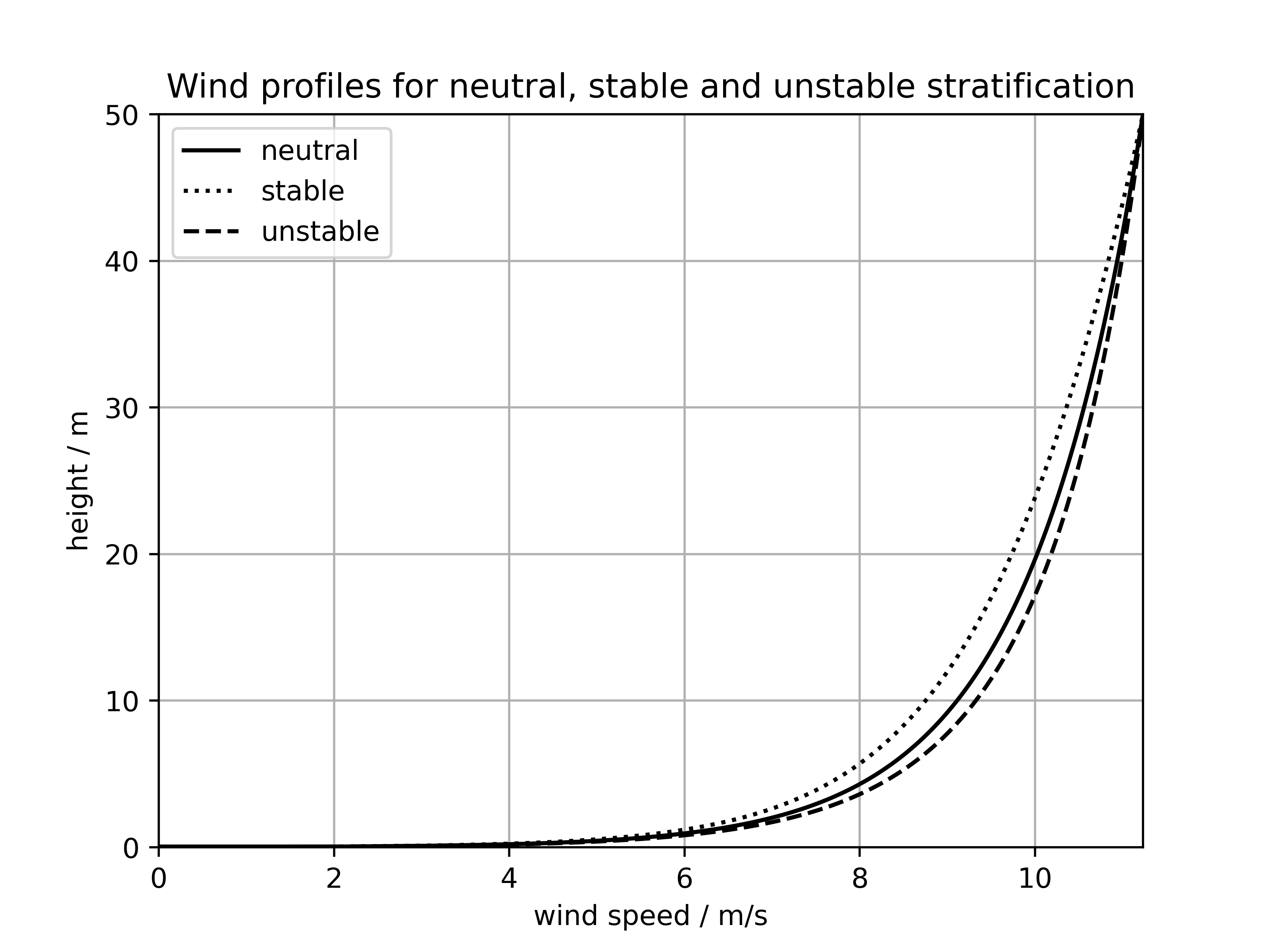
\[ \begin{align} \newoverline{u}\left(z\right) = \frac{u_\star}{k}\left[\ln\left(\frac{z}{z_0}\right) - \psi_m\left(\zeta\right)\right],\tag{17.48}\label{eq:wind_profile_pbl} \end{align} \]

$\psi_m$ is an auxiliary function that modifies the logarithmic wind profile. In the case of indifferent stratification $\psi_m = 0$. Fig. 17.1 shows with Eq. (17.48) calculated wind profiles.

The friction speed results from this:

\[ \begin{align} u_\star = \frac{Uk}{\ln\left(\frac{z}{z_0}\right) - \psi_m\left(\frac{z}{L}\right)}.\tag{17.49}\label{eq:u_star} \end{align} \]

17.3 Ekman transport

The Ekman transport occurs wherever a geostrophic medium meets a horizontal boundary at which the adhesion condition applies. Define the eddy viscosity coefficient $K$ by

\[ \begin{align} K \coloneqq \frac{A_z}{\rho}, \end{align} \]

is written Eq. (17.33) as

\[ \begin{align} \tau_{x, z} = K\rho\frac{\partial\newoverline{u}}{\partial z}. \end{align} \]

Under the assumption $\frac{\partial}{\partial z}\left(K\rho\right) = 0$, which is only a useful assumption above the Prandtl layer, holds

\[ \begin{align} \frac{1}{\rho}\frac{\partial\tau_{x, z}}{\partial z} = K\frac{\partial^2\newoverline{u}}{\partial z^2}. \end{align} \]

The equations (17.35) - (17.36) then become

\[ \begin{align} 0 = f\newtilde{v}+ K\frac{\partial^2\newoverline{u}}{\partial z^2}, & {} & 0 = -f\newtilde{u} + K\frac{\partial^2\newoverline{v}}{\partial z^2}. \end{align} \]

It became the definition

\[ \begin{align} \newtilde{u} \coloneqq \newoverline{u} - u_g, & {} & \newtilde{v} \coloneqq \newoverline{u} - v_g \end{align} \]

with $\mathbf{v}_{h, g} = \left(u_g, v_g\right)^T$ used as the geostrophic wind. If you neglect the thermal wind, it follows

\[ \begin{align} 0 = f\newtilde{v}+ K\frac{\partial^2\newtilde{u}}{\partial z^2}, & {} & 0 = -f\newtilde{u} + K\frac{\partial^2\newtilde{v}}{\partial z^2} & {} & \Rightarrow \frac{if}{K}\left(\newtilde{u} + i\newtilde{v}\right) = \frac{\partial^2\left(\newtilde{u} + i\newtilde{v}\right)}{\partial z^2}. \end{align} \]

This is solved by

\[ \begin{align} \newtilde{u} + i\newtilde{v} &= C\exp\left(\sqrt{\frac{if}{K}}z\right) + C_2\exp\left(-\sqrt{\frac{if}{K}}z\right) \end{align} \]

with $C, C_2\in \mathbb{C}$. In the case of the lower limit of the atmosphere, the boundary conditions apply in the Northern Hemisphere

\[ \begin{align} \lim_{z\to\infty}\newtilde{u} + i\newtilde{v} &= 0 \Rightarrow C = 0,\\ \left(\newtilde{u} + i\newtilde{v}\right)\left(z = 0\right) &= -u_g - iv_g \Rightarrow C_2 = -u_g - iv_g, \end{align} \]

and in the southern hemisphere

\[ \begin{align} \lim_{z\to\infty}\newtilde{u} + i\newtilde{v} &= 0 \Rightarrow C_2 = 0,\\ \left(\newtilde{u} + i\newtilde{v}\right)\left(z = 0\right) &= -u_g - iv_g \Rightarrow C = -u_g - iv_g, \end{align} \]

so the solution is north of the equator

\[ \begin{align} \newtilde{u} + i\newtilde{v} = -\left(u_g + iv_g\right)\exp\left(-\sqrt{\frac{if}{K}}z\right) = -\left(u_g + iv_g\right)\exp\left(-\sqrt{\frac{f}{2K}}z\right)\exp\left(-i\sqrt{\frac{f}{2K}}z\right) \end{align} \]

and south of it

\[ \begin{align} \newtilde{u} + i\newtilde{v} = -\left(u_g + iv_g\right)\exp\left(-\sqrt{\frac{\left|f\right|}{iK}}z\right) = -\left(u_g + iv_g\right)\exp\left(-\sqrt{\frac{\left|f\right|}{2K}}z\right)\exp\left(i\sqrt{\frac{\left|f\right|}{2K}}z\right). \end{align} \]

This can be generalized to:

\[ \begin{align} \newoverline{u} &= u_g - \left[\sign\left(f\right)v_g\sin\left(\sqrt{\frac{\left|f\right|}{2K}}z\right) + u_g\cos\left(\sqrt{\frac{\left|f\right|}{2K}}z\right)\right]\exp\left(-\sqrt{\frac{\left|f\right|}{2K}}z\right),\\ \newoverline{v} &= v_g + \left[\sign\left(f\right)u_g\sin\left(\sqrt{\frac{\left|f\right|}{2K}}z\right) - v_g\cos\left(\sqrt{\frac{\left|f\right|}{2K}}z\right)\right]\exp\left(-\sqrt{\frac{\left|f\right|}{2K}}z\right). \end{align} \]

You can o. B. d. A. Assuming $u_g > 0, v_g = 0$, then the following applies

$\sign\left(f\right)\rho\newoverline{v}$ is the mass flux density into the deep, so double partial integration is used

\[ \begin{align} \int_0^\infty\sin\left(\alpha z\right)\exp\left(-\beta z\right)dz &= \frac{\alpha}{\beta}\int_0^\infty\cos\left(\alpha z\right)\exp\left(-\beta z\right)dz = \frac{\alpha}{\beta^2} - \frac{\alpha^2}{\beta^2}\int_0^\infty\sin\left(\alpha z\right)\exp\left(-\beta z\right)dz\nonumber\\ \Rightarrow\int_0^\infty\sin\left(\alpha z\right)\exp\left(-\beta z\right)dz &= \frac{\frac{\alpha}{\beta^2}}{1 + \frac{\alpha^2}{\beta^2}} = \frac{\alpha}{\beta^2 + \alpha^2}. \end{align} \]

In an isothermal atmosphere applies

\[ \begin{align} \alpha = \sqrt{\frac{\left|f\right|}{2K}},& {} & \beta = -\sqrt{\frac{\left|f\right|}{2K}} - \frac{1}{H}\\ \Rightarrow \alpha^2 + \beta^2 = \frac{\left|f\right|}{K} + \frac{1}{H^2} + \sqrt{\frac{2\left|f\right|}{KH^2}} & {} & \Rightarrow \frac{\alpha}{\beta^2 + \alpha^2} = \frac{1}{\sqrt{\frac{2\left|f\right|}{K}} + \sqrt{\frac{2K}{\left|f\right|H^4}} + \frac{2}{H}} = \frac{H}{2 + H\sqrt{\frac{2\left|f\right|}{K}} + \sqrt{\frac{2K}{fH^2}}} \end{align} \]

with $H \approx 8$ km as the scale height. From this it follows

\[ \begin{align} \sign\left(f\right)\int_0^\infty\rho\newoverline{v}dz = \frac{H}{2 + H\sqrt{\frac{2\left|f\right|}{K}} + \sqrt{\frac{2K}{fH^2}}} \end{align} \]

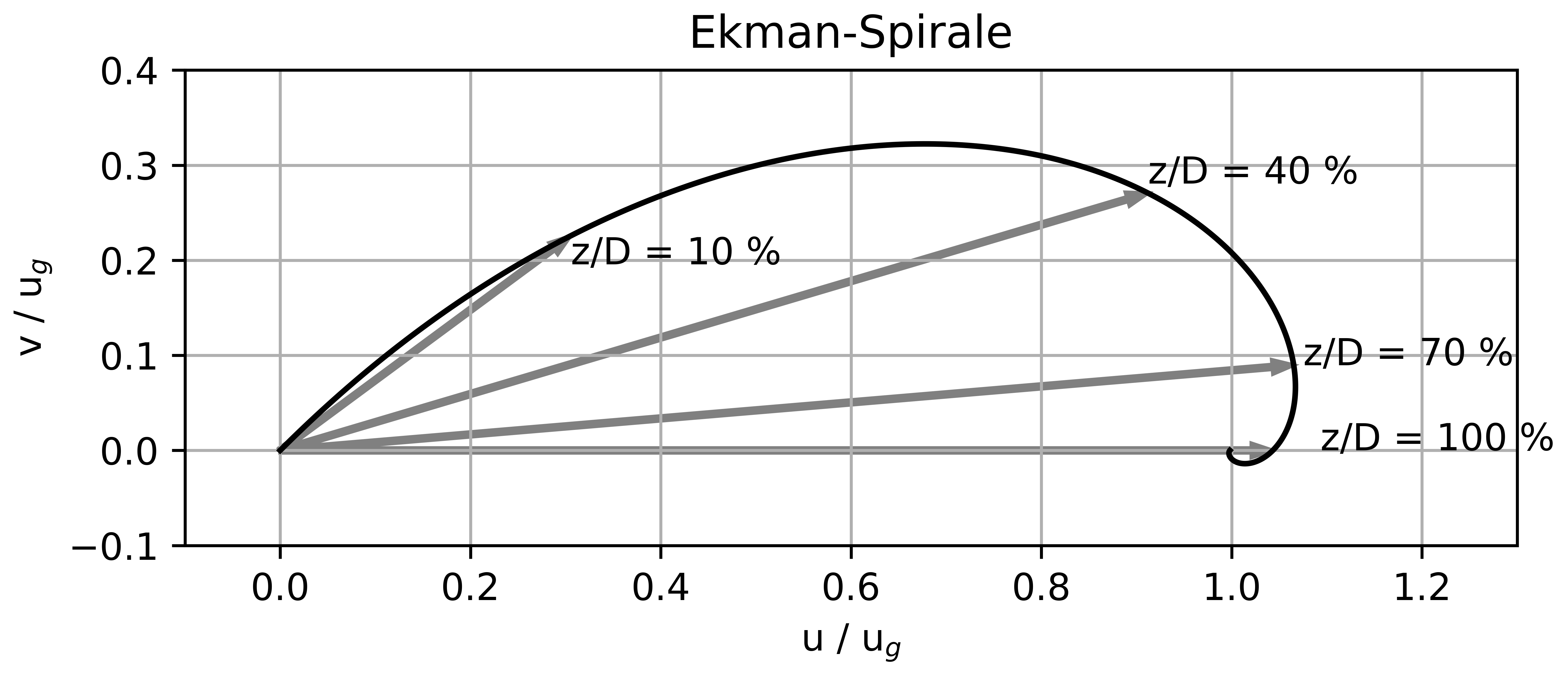
for the mass flux density into the deep. The height $D$ at which the wind is parallel to the geostrophic wind is often used as a technical definition of Boundary layer thickness. It applies

There the wind speed is slightly higher than the geostrophic speed, which is why this height is also referred to as gradient wind height.

This allows the system of equations (17.65) - (17.66) to be written in the form

note down. From observations we know that at a height of approx. 1 km the wind strives for its geostrophic value, and it follows from this

\[ \begin{align} K \approx \frac{\left|f\right|D^2}{2\pi^2} \approx 5\text{ m}^2/\text{s}.\tag{17.74}\label{sec:eddy_viscosity_vert_estimate} \end{align} \]

This is over five orders of magnitude above the kinematic viscosity value of $1.5\cdot 10^{-5}$ m$^2$/s. With Eq. (17.34) follows for the mixing path length

\[ \begin{align} l = \sqrt{\frac{K}{\left|\frac{\partial\newoverline{\mathbf{v}_h}}{\partial z}\right|}} \sim \sqrt{\frac{KD}{u_g}} \sim 2\cdot 10^1\text{ m}.\tag{17.75}\label{eq:estimate_mix_len} \end{align} \]

This corresponds to the expectation that $l \ll D$ must be for the mixing path concept to be meaningful in the planetary boundary layer. It follows from Eq. (17.40) a height $D_P$ of the Prandtl layer of approx.

\[ \begin{align} D_P = \frac{l}{k} = 50\text{ m} \end{align} \]

with $k = 0, 4$. One defines the Ekman number $\Ek$ as the ratio of friction to Coriolisterms, i.e

where $H$ is the characteristic vertical extent of the phenomenon. At small Ekman numbers, the friction force can be balanced by the Coriolis force. In the boundary layer one obtains an Ekman number of $\Ek \sim 5$ %.

For a cyclone with radius $R$, the Ekman spiral leads to a pressure tendency $\frac{\partial p}{\partial t}$ of the order of magnitude

\[ \begin{align} \frac{\partial p}{\partial t} & \sim \frac{2g}{R}\frac{u_g\rho_0\alpha}{\beta^2 + \alpha^2}. \end{align} \]

With $u_g \sim 10$ m/s, $\rho_0 \approx 1, 2$ kg/m$^3$ and $R \sim 500$ km

\[ \begin{align} \frac{\partial p}{\partial t} & \sim 2, 6\text{ }\frac{\text{hPa}}{\text{hr}}. \end{align} \]

This is significantly lower than the value estimated in Sect. 13.10.2. The upper limit of the boundary layer is also the upper limit of the Ekman layer.

17.3.1 Importance of Eddy Viscosity

Eddy exchange coefficients $A_{i, j}$ and mixing path lengths $l_x$, $l_y$, $l_z$ were introduced to examine the effects of turbulence, i.e. h. the subscale variability, to describe the resolved (averaged) fields. It is questionable how fundamental these quantities are, i.e. i.e. whether these are material properties or rather auxiliary variables.

First of all, it can be stated that at very fine resolution the diffusion coefficients describe the molecular flows, i.e. converge to the molecular physical diffusion coefficients. At a coarser resolution, however, the diffusive terms also contain turbulent components. However, in this chapter no explicit assumptions were made about the spatial or temporal scope of the averaging operators. On the other hand, it was implicitly assumed that the averaging operator is a Reynolds operator. This is only a realistic assumption if the turbulent fluctuations are small compared to the size of the averaging, but the averaging is not so extensive that synoptic-scale processes are affected. Such an averaging is, in a sense, superior to others, and so are the eddy exchange coefficients and mixing path lengths obtained with it.

17.3.2 Monin-Obukhov length

The length

\[ \begin{align} L \coloneqq -\frac{\newoverline{\theta}u_\star^3}{kg\newoverline{\left(w'\theta'\right)}}\tag{17.80}\label{eq:mo_length} \end{align} \]

is called Monin-Obukhov length.

17.3.3 Spin down

If one assumes time independence of the density, it follows from the continuity equation

\[ \begin{align} \frac{\partial}{\partial z}\left(\rho w\right) = -\frac{\partial}{\partial x}\left(\rho u\right) - \frac{\partial}{\partial y}\left(\rho v\right). \end{align} \]

Integrating this from $z = 0$ to $z = D$ under the assumption $w\left(z = 0\right) = 0$ gives

\[ \begin{align} \left(\rho w\right)_D = -\int_0^D\frac{\partial}{\partial x}\left(\rho u\right) + \frac{\partial}{\partial y}\left(\rho v\right)dz. \end{align} \]

If you put Eq. (17.73), you get

\[ \begin{align} \left(\rho w\right)_D = -\sign\left(f\right)\frac{\partial}{\partial y}\int_0^D\rho u_g\sin\left(\frac{\pi}{D}z\right)\exp\left(-\frac{\pi}{D}z\right)dz. \end{align} \]

If you assume a homogeneous density, you get from this

\[ \begin{align} w\left(D\right) = -\sign\left(f\right)\frac{\partial u_g}{\partial y}\int_0^D\sin\left(\frac{\pi}{D}z\right)\exp\left(-\frac{\pi}{D}z\right)dz. \end{align} \]

$\zeta_g = -\frac{\partial u_g}{\partial y}$ is the geostrophic vorticity, thus follows

\[ \begin{align} w\left(D\right) = \sign\left(f\right)\zeta_g\int_0^D\sin\left(\frac{\pi}{D}z\right)\exp\left(-\frac{\pi}{D}z\right)dz. \end{align} \]

Again using partial integration one obtains

\[ \begin{align} &\int_0^D\sin\left(\frac{\pi}{D}z\right)\exp\left(-\frac{\pi}{D}z\right)dz = -\left[\frac{D}{\pi}\cos\left(\frac{\pi}{D}z\right)\exp\left(-\frac{\pi}{D}z\right)\right]_0^D - \int_0^D\cos\left(\frac{\pi}{D}z\right)\exp\left(-\frac{\pi}{D}z\right)dz\nonumber\\ &= \frac{D}{\pi}\left(1 + e^{-\pi}\right) - \int_0^D\cos\left(\frac{\pi}{D}z\right)\exp\left(-\frac{\pi}{D}z\right)dz\nonumber\\ &= \frac{D}{\pi}\left(1 + e^{-\pi}\right) - \left[\frac{D}{\pi}\sin\left(\frac{\pi}{D}z\right)\exp\left(-\frac{\pi}{D}z\right)\right]_0^D - \int_0^D\sin\left(\frac{\pi}{D}z\right)\exp\left(-\frac{\pi}{D}z\right)dz\nonumber\\ &\Rightarrow \int_0^D\sin\left(\frac{\pi}{D}z\right)\exp\left(-\frac{\pi}{D}z\right)dz = \frac{D}{2\pi}\left(1 + e^{-\pi}\right) \approx \frac{D}{2\pi} = \sqrt{\frac{K}{2f}}. \end{align} \]

This implies neglecting the approximately sign

If you substitute $\zeta_g \sim 10^{-5}$, $f \sim 10^{-4}, K \sim 2$ in SI units, you get

\[ \begin{align} w \sim 0,1 \text{ cm/s}. \end{align} \]

The quasi-geostrophic vorticity equation Eq. (13.219) is with a transformation into the z system, neglecting advection

\[ \begin{align} \frac{\partial\zeta_g}{\partial t} = f\frac{\partial w}{\partial z}. \end{align} \]

If you integrate this from $D$ to the tropopause height $z_T$, you get $w\left(z = z_T\right) = 0$ under the assumption

\[ \begin{align} \int_D^{z_T}\frac{\partial\zeta_g}{\partial t}dz = -fw\left(D\right). \end{align} \]

Assuming that the geostrophic relative vorticity is height independent,

\[ \begin{align} \frac{\partial\zeta_g}{\partial t} = -\frac{f}{z_T - D}w\left(D\right). \end{align} \]

If you put Eq. (17.87), you get

\[ \begin{align} \frac{\partial\zeta_g}{\partial t} = -\frac{\zeta_g}{z_T - D}\sqrt{\frac{K\left|f\right|}{2}} \approx -\zeta_g\sqrt{\frac{K\left|f\right|}{2z_T^2}}. \end{align} \]

From this it follows, again ignoring the approximately sign,

\[ \begin{align} \zeta_g\left(t\right) = \zeta_g\left(0\right)\exp\left(-\sqrt{\frac{K\left|f\right|}{2z_T^2}}t\right) = \zeta_g\left(0\right)\exp\left(-\frac{t}{\tau}\right) \end{align} \]

with the spin-down time

If you substitute $z_T \sim 10^4$, $f \sim 10^{-4}, K \sim 2$ in SI units, you get

\[ \begin{align} \tau \sim 10^6\text{ s} \sim 10\text{ d}. \end{align} \]

17.4 Isotropic turbulence

17.4.1 Spectral form of the Navier-Stokes equations

For the Fourier transformation $\newtilde{\mathbf{v}}\left(\mathbf{k}, t\right)$ of a velocity field $\mathbf{v} = \mathbf{v}\left(\mathbf{r}, t\right)$ applies

\[ \begin{align} \newtilde{\mathbf{v}}\left(\mathbf{k}, t\right) = C^3\int_{\mathbb{R}^3}\mathbf{v}\left(\mathbf{r}, t\right)\exp\left(-i\mathbf{k}\cdot\mathbf{r}\right)d^3r. \end{align} \]

The inverse Fourier transform is

\[ \begin{align} \mathbf{v}\left(\mathbf{r}, t\right) = \newtilde{C}^3\int_{\mathbb{R}^3}\newtilde{\mathbf{v}}\left(\mathbf{k}, t\right)\exp\left(i\mathbf{k}\cdot\mathbf{r}\right)d^3k.\tag{17.97}\label{eq:velocity_field_ft_inv} \end{align} \]

At this point you set $\newtilde{C} = 1 \stackrel{\href{ch-41-orthogonal-function-systems.html#eq:ft_norm}{\text{Eq. (C.9)}}}{\Leftrightarrow} C = \frac{1}{2\pi}$ to shorten the notation and neglects the $\mathbb{R}^3$ on the integral. The incompressible momentum equation is:

\[ \begin{align} \frac{\partial\mathbf{v}}{\partial t} = -\nabla\pi - \nabla\varphi - \left(\mathbf{v}\cdot\nabla\right)\mathbf{v} + \nu\Delta\mathbf{v}, \end{align} \]

where the abbreviation

\[ \begin{align} \pi\coloneqq\frac{p}{\rho} \end{align} \]

was used. The inverse Fourier transformations of the other occurring fields are:

\[ \begin{align} \pi\left(\mathbf{r}, t\right) &= \int\newtilde{\pi}\left(\mathbf{k}, t\right)\exp\left(i\mathbf{k}\cdot\mathbf{r}\right)d^3k,\\ \varphi\left(\mathbf{r}\right) &= \int\newtilde{\varphi}\left(\mathbf{k}\right)\exp\left(i\mathbf{k}\cdot\mathbf{r}\right)d^3k. \end{align} \]

This also applies to the application of the differential operators to the fields

\[ \begin{align} \frac{\partial\mathbf{v}}{\partial t} &= \int\frac{\partial\newtilde{\mathbf{v}}\left(\mathbf{k}, t\right)}{\partial t}\exp\left(i\mathbf{k}\cdot\mathbf{r}\right)d^3k,\\ -\nabla\pi &= -i\int\mathbf{k}\newtilde{\pi}\left(\mathbf{k}, t\right)\exp\left(i\mathbf{k}\cdot\mathbf{r}\right)d^3k,\\ -\nabla\varphi &= -i\int\mathbf{k}\newtilde{\varphi}\left(\mathbf{k}\right)\exp\left(i\mathbf{k}\cdot\mathbf{r}\right)d^3k,\\ \Delta\mathbf{v} &= -\int\mathbf{k}^2\newtilde{\mathbf{v}}\left(\mathbf{k}, t\right)\exp\left(i\mathbf{k}\cdot\mathbf{r}\right)d^3k. \end{align} \]

applies to momentum advection

\[ \begin{align} \left(\mathbf{v}\cdot\nabla\right)\mathbf{v} &= \left(\int\newtilde{\mathbf{v}}\left(\mathbf{k}, t\right)\exp\left(i\mathbf{k}\cdot\mathbf{r}\right)d^3k\cdot\nabla\right)\int\newtilde{\mathbf{v}}\left(\mathbf{k}, t\right)\exp\left(i\mathbf{k}\cdot\mathbf{r}\right)d^3k\nonumber\\ &= \left(\int\newtilde{\mathbf{v}}\left(\mathbf{k}', t\right)\exp\left(i\mathbf{k}'\cdot\mathbf{r}\right)d^3k'\cdot\nabla\right)\int\newtilde{\mathbf{v}}\left(\mathbf{k}'', t\right)\exp\left(i\mathbf{k}''\cdot\mathbf{r}\right)d^3k''\nonumber\\ &= \int\int\exp\left(i\mathbf{k}'\cdot\mathbf{r}\right)\left[\newtilde{\mathbf{v}}\left(\mathbf{k}', t\right)\cdot\nabla\right]\left[\newtilde{\mathbf{v}}\left(\mathbf{k}'', t\right)\exp\left(i\mathbf{k}''\cdot\mathbf{r}\right)\right]d^3k'd^3k''\nonumber\\ &= i\int\int\left[\newtilde{\mathbf{v}}\left(\mathbf{k}', t\right)\cdot\mathbf{k}''\right]\newtilde{\mathbf{v}}\left(\mathbf{k}'', t\right)\exp\left[i\left(\mathbf{k}' + \mathbf{k}''\right)\cdot\mathbf{r}\right]d^3k'd^3k''. \end{align} \]

This implies

\[ \begin{align} \left[\newtilde{\left(\mathbf{v}\cdot\nabla\right)\mathbf{v}}\right]\left(\mathbf{k}\right) &= \frac{i}{\left(2\pi\right)^3}\int\int\left[\newtilde{\mathbf{v}}\left(\mathbf{k}', t\right)\cdot\mathbf{k}''\right]\newtilde{\mathbf{v}}\left(\mathbf{k}'', t\right)\exp\left[i\left(-\mathbf{k} + \mathbf{k}' + \mathbf{k}''\right)\cdot\mathbf{r}\right]d^3k'd^3k''\nonumber\\ & \stackrel{\href{ch-39-derivations-of-some-mathematical-formula.html#eq:delta_distribution_prop_2}{\text{Glg. (A.84)}}}{=} i\int\int\left[\newtilde{\mathbf{v}}\left(\mathbf{k}', t\right)\cdot\mathbf{k}''\right]\newtilde{\mathbf{v}}\left(\mathbf{k}'', t\right)\delta\left(\mathbf{k}' + \mathbf{k}'' - \mathbf{k}\right)d^3k'd^3k''\nonumber\\ &= i\int\left[\newtilde{\mathbf{v}}\left(\mathbf{k}', t\right)\cdot\left(\mathbf{k} - \mathbf{k}'\right)\right]\newtilde{\mathbf{v}}\left(\mathbf{k} - \mathbf{k}', t\right)d^3k' \end{align} \]

From the incompressible continuity equation

\[ \begin{align} \nabla\cdot\mathbf{v} = 0 \end{align} \]

follows

This gives you

\[ \begin{align} \left[\newtilde{\left(\mathbf{v}\cdot\nabla\right)\mathbf{v}}\right]\left(\mathbf{k}\right) &= i\int\left[\newtilde{\mathbf{v}}\left(\mathbf{k}', t\right)\cdot\mathbf{k}\right]\newtilde{\mathbf{v}}\left(\mathbf{k} - \mathbf{k}', t\right)d^3k' \end{align} \]

From the previous calculations one can put together the development of the momentum equation with respect to plane waves:

\[ \begin{align} & \int\left(\frac{\partial}{\partial t} + \nu\mathbf{k}^2\right)\newtilde{\mathbf{v}}\left(\mathbf{k}, t\right)\exp\left(i\mathbf{k}\cdot\mathbf{r}\right)d^3k\nonumber\\ &= i\int\left\{-\mathbf{k}\newtilde{\pi}\left(\mathbf{k}, t\right) - \mathbf{k}\newtilde{\varphi}\left(\mathbf{k}\right) - \int\left[\newtilde{\mathbf{v}}\left(\mathbf{k}', t\right)\cdot\mathbf{k}\right]\newtilde{\mathbf{v}}\left(\mathbf{k} - \mathbf{k}', t\right)d^3k'\right\}\exp\left(i\mathbf{k}\cdot\mathbf{r}\right)d^3k \end{align} \]

This must apply at every point in spectral space, so

This is the spectral form of the incompressible momentum equation. From this it can be seen that the only term that contains interactions between scales is momentum advection.

17.4.2 Energy transfer function

How to get from the Parseval identity Eq. (C.31) can conclude, the specific kinetic energy with the wave vector $\mathbf{k}$ is determined by the size

\[ \begin{align} \newtilde{e}\left(\mathbf{k}, t\right) = \frac{1}{2}\newtilde{\mathbf{v}}\left(\mathbf{k}, t\right)\newtilde{\mathbf{v}}\left(-\mathbf{k}, t\right) \end{align} \]

described. If you write down Eq. (17.112) with the substitution $\mathbf{k} \to -\mathbf{k}$, one obtains

\[ \begin{align} \left(\frac{\partial}{\partial t} + \nu\mathbf{k}^2\right)\newtilde{\mathbf{v}}\left(-\mathbf{k}, t\right) &= i\mathbf{k}\newtilde{\pi}\left(-\mathbf{k}, t\right) + i\mathbf{k}\newtilde{\varphi}\left(-\mathbf{k}\right) + i\int\left[\newtilde{\mathbf{v}}\left(\mathbf{k}', t\right)\cdot\mathbf{k}\right]\newtilde{\mathbf{v}}\left(-\mathbf{k} - \mathbf{k}', t\right)d^3k'.\tag{17.114}\label{eq:deriv_turbulence_spec_0} \end{align} \]

If you multiply Eq. (17.114) with $\newtilde{\mathbf{v}}\left(\mathbf{k}, t\right)$ and takes Eq. (17.109), you get

\[ \begin{align} \newtilde{\mathbf{v}}\left(\mathbf{k}, t\right)\cdot\left(\frac{\partial}{\partial t} + \nu\mathbf{k}^2\right)\newtilde{\mathbf{v}}\left(-\mathbf{k}, t\right) &= i\int\left[\newtilde{\mathbf{v}}\left(\mathbf{k}', t\right)\cdot\mathbf{k}\right]\left[\newtilde{\mathbf{v}}\left(\mathbf{k}, t\right)\cdot\newtilde{\mathbf{v}}\left(-\mathbf{k} - \mathbf{k}', t\right)\right]d^3k'.\tag{17.115}\label{eq:deriv_turbulence_spec_1} \end{align} \]

If you multiply analogously to Eq. (17.112) with $\newtilde{\mathbf{v}}\left(-\mathbf{k}, t\right)$, one obtains

\[ \begin{align} \newtilde{\mathbf{v}}\left(-\mathbf{k}, t\right)\cdot\left(\frac{\partial}{\partial t} + \nu\mathbf{k}^2\right)\newtilde{\mathbf{v}}\left(\mathbf{k}, t\right) &= -i\int\left[\newtilde{\mathbf{v}}\left(\mathbf{k}', t\right)\cdot\mathbf{k}\right]\left[\newtilde{\mathbf{v}}\left(-\mathbf{k}, t\right)\cdot\newtilde{\mathbf{v}}\left(\mathbf{k} - \mathbf{k}', t\right)\right]d^3k'\tag{17.116}\label{eq:deriv_turbulence_spec_2} \end{align} \]

If you add the equations (17.115) and (17.116) and divide by two, you get

\[ \begin{align} & \left(\frac{\partial}{\partial t} + 2\nu\mathbf{k}^2\right)\newtilde{e}\left(\mathbf{k}, t\right)\nonumber\\ &= \frac{i}{2}\int\left[\newtilde{\mathbf{v}}\left(\mathbf{k}', t\right)\cdot\mathbf{k}\right]\left[\newtilde{\mathbf{v}}\left(\mathbf{k}, t\right)\cdot\newtilde{\mathbf{v}}\left(-\mathbf{k} - \mathbf{k}', t\right)\right]d^3k' - \frac{i}{2}\int\left[\newtilde{\mathbf{v}}\left(\mathbf{k}', t\right)\cdot\mathbf{k}\right]\left[\newtilde{\mathbf{v}}\left(-\mathbf{k}, t\right)\cdot\newtilde{\mathbf{v}}\left(\mathbf{k} - \mathbf{k}', t\right)\right]d^3k'. \end{align} \]

If you substitute in the first integral with $\mathbf{f}\left(\mathbf{k}'\right) = \mathbf{k}' - \mathbf{k}$ and in the second integral with $\mathbf{f}\left(\mathbf{k}'\right) = \mathbf{k} - \mathbf{k}'$, you get

\[ \begin{align} & \left(\frac{\partial}{\partial t} + 2\nu\mathbf{k}^2\right)\newtilde{e}\left(\mathbf{k}, t\right)\nonumber\\ &= \frac{i}{2}\int\left\{\left[\newtilde{\mathbf{v}}\left(\mathbf{k}' - \mathbf{k}, t\right)\cdot\mathbf{k}\right]\left[\newtilde{\mathbf{v}}\left(\mathbf{k}, t\right)\cdot\newtilde{\mathbf{v}}\left(-\mathbf{k}', t\right)\right] - \left[\newtilde{\mathbf{v}}\left(\mathbf{k} - \mathbf{k}', t\right)\cdot\mathbf{k}\right]\left[\newtilde{\mathbf{v}}\left(-\mathbf{k}, t\right)\cdot\newtilde{\mathbf{v}}\left(\mathbf{k}', t\right)\right]\right\}d^3k'. \end{align} \]

In the second integral, it should be noted that the minus sign that results from exchanging the integration limits cancels out the one that results from the derivation of the substituted function. One defines the energy transfer function $W = W\left(\mathbf{k}, \mathbf{k}', t\right)$ by

\[ \begin{align} W\left(\mathbf{k}, \mathbf{k}', t\right) &\coloneqq \frac{i\mathbf{k}}{2}\cdot\left\{\newtilde{\mathbf{v}}\left(\mathbf{k}' - \mathbf{k}, t\right)\left[\newtilde{\mathbf{v}}\left(\mathbf{k}, t\right)\cdot\newtilde{\mathbf{v}}\left(-\mathbf{k}', t\right)\right] - \newtilde{\mathbf{v}}\left(\mathbf{k} - \mathbf{k}', t\right)\left[\newtilde{\mathbf{v}}\left(-\mathbf{k}, t\right)\cdot\newtilde{\mathbf{v}}\left(\mathbf{k}', t\right)\right]\right\}.\tag{17.119}\label{eq:def_energy_tranfer_function} \end{align} \]

This gives you the balance equation of the kinetic energy in spectral form

This shows that the friction $\propto\frac{1}{L^2}$ is scale-sensitive and in any case reduces the spectral specific kinetic energy. For the energy transfer function applies

\[ \begin{align} W\left(\mathbf{k}', \mathbf{k}, t\right) &= \frac{i\mathbf{k}'}{2}\cdot\left\{\newtilde{\mathbf{v}}\left(\mathbf{k} - \mathbf{k}', t\right)\left[\newtilde{\mathbf{v}}\left(\mathbf{k}', t\right)\cdot\newtilde{\mathbf{v}}\left(-\mathbf{k}, t\right)\right] - \newtilde{\mathbf{v}}\left(\mathbf{k}' - \mathbf{k}, t\right)\left[\newtilde{\mathbf{v}}\left(-\mathbf{k}', t\right)\cdot\newtilde{\mathbf{v}}\left(\mathbf{k}, t\right)\right]\right\}\nonumber\\ &= -\frac{i\mathbf{k}'}{2}\cdot\left\{\newtilde{\mathbf{v}}\left(\mathbf{k}' - \mathbf{k}, t\right)\left[\newtilde{\mathbf{v}}\left(-\mathbf{k}', t\right)\cdot\newtilde{\mathbf{v}}\left(\mathbf{k}, t\right)\right] - \newtilde{\mathbf{v}}\left(\mathbf{k} - \mathbf{k}', t\right)\left[\newtilde{\mathbf{v}}\left(\mathbf{k}', t\right)\cdot\newtilde{\mathbf{v}}\left(-\mathbf{k}, t\right)\right]\right\}\nonumber\\ &= -\frac{i\mathbf{k}'}{2}\cdot\left\{\newtilde{\mathbf{v}}\left(\mathbf{k}' - \mathbf{k}, t\right)\left[\newtilde{\mathbf{v}}\left(\mathbf{k}, t\right)\cdot\newtilde{\mathbf{v}}\left(-\mathbf{k}', t\right)\right] - \newtilde{\mathbf{v}}\left(\mathbf{k} - \mathbf{k}', t\right)\left[\newtilde{\mathbf{v}}\left(-\mathbf{k}, t\right)\cdot\newtilde{\mathbf{v}}\left(\mathbf{k}', t\right)\right]\right\} \end{align} \]

From this it follows

\[ \begin{align} & W\left(\mathbf{k}', \mathbf{k}, t\right) + W\left(\mathbf{k}, \mathbf{k}', t\right)\nonumber\\ &= \frac{i\mathbf{k}}{2}\cdot\left\{\newtilde{\mathbf{v}}\left(\mathbf{k}' - \mathbf{k}, t\right)\left[\newtilde{\mathbf{v}}\left(\mathbf{k}, t\right)\cdot\newtilde{\mathbf{v}}\left(-\mathbf{k}', t\right)\right] - \newtilde{\mathbf{v}}\left(\mathbf{k} - \mathbf{k}', t\right)\left[\newtilde{\mathbf{v}}\left(-\mathbf{k}, t\right)\cdot\newtilde{\mathbf{v}}\left(\mathbf{k}', t\right)\right]\right\}\nonumber\\ & - \frac{i\mathbf{k}'}{2}\cdot\left\{\newtilde{\mathbf{v}}\left(\mathbf{k}' - \mathbf{k}, t\right)\left[\newtilde{\mathbf{v}}\left(\mathbf{k}, t\right)\cdot\newtilde{\mathbf{v}}\left(-\mathbf{k}', t\right)\right] - \newtilde{\mathbf{v}}\left(\mathbf{k} - \mathbf{k}', t\right)\left[\newtilde{\mathbf{v}}\left(-\mathbf{k}, t\right)\cdot\newtilde{\mathbf{v}}\left(\mathbf{k}', t\right)\right]\right\}\nonumber\\ &= \frac{i}{2}\left[\newtilde{\mathbf{v}}\left(\mathbf{k}, t\right)\cdot\newtilde{\mathbf{v}}\left(-\mathbf{k}', t\right)\right]\newtilde{\mathbf{v}}\left(\mathbf{k}' - \mathbf{k}, t\right)\cdot\left(\mathbf{k} - \mathbf{k}'\right)\nonumber\\ & -\frac{i}{2}\left[\newtilde{\mathbf{v}}\left(-\mathbf{k}, t\right)\cdot\newtilde{\mathbf{v}}\left(\mathbf{k}', t\right)\right]\newtilde{\mathbf{v}}\left(\mathbf{k} - \mathbf{k}', t\right)\cdot\left(\mathbf{k} - \mathbf{k}'\right)\nonumber\\ & \stackrel{\href{#eq:cont_incom_spec}{\text{Glg. (17.109)}}}{=} 0. \end{align} \]

The energy transfer function is therefore antisymmetric:

This is related to the conservation of energy: the energy gain of component $\mathbf{k}$ at the expense of component $\mathbf{k}'$ is equal to the energy loss of component $\mathbf{k}'$ due to component $\mathbf{k}$.

17.4.2.1 Isotropic form

Now one makes the assumption of isotropy, i.e. h. It is assumed that spectral properties do not depend on the three components of the vector $\mathbf{k}$, but only on the magnitude of $k$, i.e

\[ \begin{align} e\left(\mathbf{k}, t\right) \to \frac{\newtilde{e}\left(k, t\right)}{4\pi k^2}, & {} & W\left(\mathbf{k}, \mathbf{k}, t\right) \to \frac{W\left(k, k', t\right)}{4\pi k'^24\pi k^2}. \end{align} \]

The geometry of the spherical coordinates was corrected. Thus, Eq. (17.120) to

\[ \begin{align} \left(\frac{\partial}{\partial t} + 2\nu k^2\right)\frac{\newtilde{e}\left(k, t\right)}{4\pi k^2} &= \int\frac{W\left(k, k', t\right)}{4\pi k'^24\pi k^2}4\pi k'^2dk'\nonumber \end{align} \]

17.4.3 Heisenberg approach

The Heisenberg approach initially assumes stationarity, i.e

\[ \begin{align} 2\nu k^2\newtilde{e}\left(k\right) &= \int W\left(k, k'\right)dk'.\tag{17.126}\label{eq:heisenberg_turb_0} \end{align} \]

Furthermore, it is assumed that there is a cutoff wave number $k^\star$, which divides the spectrum into two regions:

• The region $k < k^\star$ (larger wavelengths) is referred to as region 1. For geometric reasons, no isotropy can be assumed here. The Heisenberg approach makes no statements about this area.
• The region $k \geq k^\star$ (smaller wavelengths) is called universality region. Isotropy can be assumed here and the flow is little influenced by boundary conditions.

The Heisenberg approach refers exclusively to the universality region. It is assumed that the smaller scales have a similar effect on the larger scales as the viscosity has on the smallest-scale vortices: they diffuse momentum. This is justified because it can be assumed that the smaller-scale vortices diffuse momentum on average (reduce the gradient of the velocity field). The Heisenberg approach is the formula

\[ \begin{align} W\left(k, k'\right) = -2\kappa_Hk^2\newtilde{e}\left(k\right)g\left(k', \newtilde{e}\left(k'\right)\right), \end{align} \]

where $k, k' \geq k^\star$ and $k' > k$ are assumed.

\[ \begin{align} \kappa_H = 0,5\pm 0,03\tag{17.128}\label{eq:heisenberg_constant_value} \end{align} \]

[13] is a kind of dimensionless viscosity, the so-called Heisenberg constant. This formula is analogous to the molecular dissipative term $-2\nu k^2\newtilde{e}\left(k\right)$. The function $g\left(k', \newtilde{e}\left(k'\right)\right)$ describes how the smaller scale $k'$ acts on the scale $k$, whereby an explicit dependence on the energy $\newtilde{e}\left(k'\right)$ present at $k'$ was included. Apply in the SI system

\[ \begin{align} \left[\newtilde{e}\right] &= \frac{\text{J}}{\text{kg/m}} = \frac{\text{Jm}}{\text{kg}} = \frac{\text{Nm}^2}{\text{kg}} = \frac{\text{m}^3}{\text{s}^2}\\ \Rightarrow \left[\frac{\partial\newtilde{e}}{\partial t}\right] = \frac{\text{m}^3}{\text{s}^3}, & {} & \left[W\right] = \frac{\text{m}^4}{\text{s}^3}, & {} & \Rightarrow \left[k^2\newtilde{e}\left(k\right)\right] = \frac{\text{m}}{\text{s}^2} & {} & \Rightarrow \left[g\left(k', \newtilde{e}\left(k'\right)\right)\right] = \frac{\text{m}^3}{\text{s}}. \end{align} \]

The approach for $g$ is now chosen

\[ \begin{align} g\left(k', \newtilde{e}\left(k'\right)\right) = \left(k'\right)^\alpha\newtilde{e}\left(k'\right)^\beta. \end{align} \]

This implies

\[ \begin{align} \beta &= \frac{1}{2}, \alpha = -\frac{3}{2}\\ \Rightarrow g\left(k', \newtilde{e}\left(k'\right)\right) &= \left(k'\right)^{-3/2}\newtilde{e}\left(k'\right)^{1/2} = \sqrt{\frac{\newtilde{e}\left(k'\right)}{\left(k'\right)^3}}. \end{align} \]

In summary, the Heisenberg approach is

\[ \begin{align} T\left(k, k'\right) = \begin{cases} -2\kappa_Hk^2\newtilde{e}\left(k\right)\newtilde{e}\left(k'\right)^{1/2}\left(k'\right)^{-3/2},\text{ falls }k' \geq k\text{ gilt (Energieverlust an kleinere Skala),}\\ 2\kappa_Hk^2\newtilde{e}\left(k\right)\newtilde{e}\left(k'\right)^{1/2}\left(k'\right)^{-3/2},\text{ falls }k' < k\text{ gilt (Energiegewinn von größerer Skala).} \end{cases}\tag{17.134}\label{eq:heisenberg-ansatz} \end{align} \]

In the context of stationarity, the kinetic energy lost through dissipation is compensated by the supply from the larger scales. The larger scales therefore have an energy loss to the smaller scales, which must be compensated for by a production $\sigma\left(k\right)$ of kinetic energy. The mechanism through which this happens is left open here. However, one assumes $\sigma\left(k\right) = 0$ for $k > k^\star$ in order to simplify the considerations in the universality region. Eq. (17.126) becomes

\[ \begin{align} 2\nu k^2\newtilde{e}\left(k\right) &= \int W\left(k, k'\right)dk' + \sigma\left(k\right).\tag{17.135}\label{eq:heisenberg_turb_1} \end{align} \]

17.4.4 Energy spectrum

If you integrate Eq. (17.135) up to a wave number $k > k^\star$, one obtains

\[ \begin{align} 2\nu\int_0^k\left(k'\right)^2\newtilde{e}\left(k'\right)dk' &= \int_0^k\int_0^\infty W\left(k', k''\right)dk''dk' + \int_0^k\sigma\left(k'\right)dk'.\tag{17.136}\label{eq:heisenberg_turb_2} \end{align} \]

For $k = \infty$ one obtains

\[ \begin{align} 2\nu\int_0^\infty\left(k'\right)^2\newtilde{e}\left(k'\right)dk' &= \int_0^\infty\int_0^\infty W\left(k', k''\right)dk''dk' + \int_0^\infty\sigma\left(k'\right)dk'. \end{align} \]

Due to the antisymmetry of the energy transfer function $W\left(k', k''\right) = -W\left(k'', k'\right)$ holds

\[ \begin{align} \int_0^\infty\int_0^\infty W\left(k', k''\right)dk''dk' = 0. \end{align} \]

This corresponds to the fact that the energy transfer function redistributes kinetic energy, but does not produce or destroy kinetic energy. This leads to

\[ \begin{align} 2\nu\int_0^\infty\left(k'\right)^2\newtilde{e}\left(k'\right)dk' = \int_0^\infty\sigma\left(k'\right)dk'. \end{align} \]

This corresponds to the fact that under stationary conditions the energy input is equal to the energy loss. The energy loss is equal to the dissipation:

\[ \begin{align} \epsilon = 2\nu\int_0^\infty\left(k'\right)^2\newtilde{e}\left(k'\right)dk' \end{align} \]

Because $k > k^\star$ and $\sigma\left(k'\right) = 0$ for $k' > k^\star$ holds

\[ \begin{align} \int_0^k\sigma\left(k'\right)dk' = \int_0^\infty\sigma\left(k'\right)dk'. \end{align} \]

Thus, one can use Eq. (17.136) in the form

\[ \begin{align} 2\nu\int_0^k\left(k'\right)^2\newtilde{e}\left(k'\right)dk' &= \int_0^k\int_0^\infty W\left(k', k''\right)dk''dk' + \epsilon \end{align} \]

write down. Again because of the antisymmetry $W\left(k', k''\right) = -W\left(k'', k'\right)$ holds

\[ \begin{align} \int_0^k\int_0^kW\left(k', k''\right)dk''dk' = 0. \end{align} \]

Therefore applies

\[ \begin{align} 2\nu\int_0^k\left(k'\right)^2\newtilde{e}\left(k'\right)dk' &= \int_0^k\int_k^\infty W\left(k', k''\right)dk''dk' + \epsilon\nonumber\\ \Leftrightarrow \epsilon &= 2\nu\int_0^k\left(k'\right)^2\newtilde{e}\left(k'\right)dk' - \int_0^k\int_k^\infty W\left(k', k''\right)dk''dk''. \end{align} \]

If you put Eq. (17.134) and consider $k'' > k'$, you get

\[ \begin{align} \epsilon &= 2\nu\int_0^k\left(k'\right)^2\newtilde{e}\left(k'\right)dk' - \int_0^k\int_k^\infty-2\kappa_H\left(k'\right)^2\newtilde{e}\left(k'\right)\newtilde{e}\left(k''\right)^{1/2}\left(k''\right)^{-3/2}dk''dk'\nonumber\\ \Leftrightarrow \epsilon &= 2\nu\int_0^k\left(k'\right)^2\newtilde{e}\left(k'\right)dk' + 2\kappa_H\int_0^k\int_k^\infty\left(k'\right)^2\newtilde{e}\left(k'\right)\newtilde{e}\left(k''\right)^{1/2}\left(k''\right)^{-3/2}dk''dk'\nonumber\\ \Leftrightarrow \epsilon &= 2\nu\int_0^k\left(k'\right)^2\newtilde{e}\left(k'\right)dk' + 2\kappa_H\int_k^\infty\newtilde{e}\left(k''\right)^{1/2}\left(k''\right)^{-3/2}dk''\int_0^k\left(k'\right)^2\newtilde{e}\left(k'\right)dk'\nonumber\\ \Leftrightarrow \epsilon &= 2\nu\int_0^k\left(k'\right)^2\newtilde{e}\left(k'\right)dk' + 2\kappa_H\int_k^\infty\sqrt{\frac{\newtilde{e}\left(k''\right)}{\left(k''\right)^3}}dk''\int_0^k\left(k'\right)^2\newtilde{e}\left(k'\right)dk'\nonumber\\ \Leftrightarrow\epsilon &= \left(2\nu + 2\kappa_H\int_k^\infty\sqrt{\frac{\newtilde{e}\left(k''\right)}{\left(k''\right)^3}}dk''\right)\int_0^k\left(k'\right)^2\newtilde{e}\left(k'\right)dk'\nonumber\\ \Leftrightarrow\epsilon &= \left(\nu + \kappa_H\int_k^\infty\sqrt{\frac{\newtilde{e}\left(k''\right)}{\left(k''\right)^3}}dk''\right)\int_0^k2\left(k'\right)^2\newtilde{e}\left(k'\right)dk'.\tag{17.145}\label{eq:heisenberg_turb_3} \end{align} \]

The size

\[ \begin{align} K \coloneqq \kappa_H\int_k^\infty\sqrt{\frac{\newtilde{e}\left(k'\right)}{\left(k'\right)^3}}dk'\tag{17.146}\label{eq:heisenberg_exchange} \end{align} \]

has the dimension of a viscosity and is called Heisenberg's exchange coefficient.

You now define an auxiliary function

\[ \begin{align} f\left(k\right) \coloneqq 2\int_0^k\left(k'\right)^2\newtilde{e}\left(k'\right)dk' \Rightarrow f'\left(k\right) = 2k^2\newtilde{e}\left(k\right).\tag{17.147}\label{eq:heisenberg_turb_6} \end{align} \]

This allows Eq. (17.145) in the form

\[ \begin{align} \frac{\epsilon}{f\left(k\right)} = \nu + \kappa_H\int_k^\infty\sqrt{\frac{\newtilde{e}\left(k'\right)}{\left(k'\right)^3}}dk' = \nu + \kappa_H\int_k^\infty\sqrt{\frac{f'\left(k'\right)}{2\left(k'\right)^5}}dk'\tag{17.148}\label{eq:heisenberg_turb_5} \end{align} \]

note down. If you differentiate this equation, you get

\[ \begin{align} -\frac{\epsilon f'\left(k\right)}{f\left(k\right)^2} = -\kappa_H\sqrt{\frac{f'\left(k\right)}{2k^5}} \Rightarrow \frac{\epsilon^2f'\left(k\right)^2}{f\left(k\right)^4} = \kappa_H^2\frac{f'\left(k\right)}{2k^5} \Leftrightarrow \frac{\epsilon^2f'\left(k\right)}{f\left(k\right)^4} = \frac{\kappa_H^2}{2k^5}. \end{align} \]

If you integrate both sides over $k$, you get

\[ \begin{align} -\frac{\epsilon^2}{3f\left(k\right)^3} + C = -\frac{\kappa_H^2}{8k^4} \Leftrightarrow \frac{\epsilon^2}{3f\left(k\right)^3} = C + \frac{\kappa_H^2}{8k^4}\tag{17.150}\label{eq:heisenberg_turb_4} \end{align} \]

with an integration constant $C$. To determine this, consider Eq. (17.150) for $k \to \infty$:

\[ \begin{align} C = \frac{\epsilon^2}{3f\left(\infty\right)^3} \end{align} \]

To determine $f\left(\infty\right)$, evaluate Eq. (17.148) for $k \to \infty$ from:

\[ \begin{align} \frac{\epsilon}{f\left(\infty\right)} &= \nu \Rightarrow f\left(\infty\right) = \frac{\epsilon}{\nu}\nonumber\\ \Rightarrow C &= \frac{\epsilon^2}{3f\left(\infty\right)^3} = \frac{\nu^3}{3\epsilon} \end{align} \]

Putting this into Eq. (17.150), you get

\[ \begin{align} \frac{\epsilon^2}{3f\left(k\right)^3} &= \frac{\nu^3}{3\epsilon} + \frac{\kappa_H^2}{8k^4}\nonumber\\ \Rightarrow f\left(k\right)^3 &= \frac{\epsilon^2}{3}\left(\frac{\kappa_H^2}{8k^4} + \frac{\nu^3}{3\epsilon}\right)^{-1}\nonumber\\ \Rightarrow f\left(k\right) &= \frac{\epsilon^{2/3}}{3^{1/3}}\left(\frac{\kappa_H^2}{8k^4} + \frac{\nu^3}{3\epsilon}\right)^{-1/3}. \end{align} \]

If you differentiate this by $k$, you get

\[ \begin{align} f'\left(k\right) &= \frac{\epsilon^{2/3}}{3^{1/3}}\frac{4}{3}\frac{\kappa_H^2}{8k^5}\left(\frac{\kappa_H^2}{8k^4} + \frac{\nu^3}{3\epsilon}\right)^{-4/3}. \end{align} \]

If you put Eq. (17.147), you get

\[ \begin{align} 2k^2\newtilde{e}\left(k\right) &= \frac{\epsilon^{2/3}}{3^{1/3}}\frac{4}{3}\frac{\kappa_H^2}{8k^5}\left(\frac{\kappa_H^2}{8k^4} + \frac{\nu^3}{3\epsilon}\right)^{-4/3}\nonumber\\ \Leftrightarrow \newtilde{e}\left(k\right) &= \frac{\epsilon^{2/3}}{3^{1/3}}\frac{2}{3k^3}\frac{\kappa_H^2}{8k^4}\left(\frac{\kappa_H^2}{8k^4} + \frac{\nu^3}{3\epsilon}\right)^{-4/3}\nonumber\\ \Leftrightarrow \newtilde{e}\left(k\right) &= \frac{\epsilon^{2/3}}{3^{1/3}}\frac{2}{3k^3}\left(\frac{\kappa_H^2}{8k^4}\right)^{-1/3}\left(\frac{8k^4}{\kappa_H^2}\right)^{-4/3}\left(\frac{\kappa_H^2}{8k^4} + \frac{\nu^3}{3\epsilon}\right)^{-4/3}\nonumber\\ \Leftrightarrow \newtilde{e}\left(k\right) &= \frac{\epsilon^{2/3}}{3^{1/3}}\frac{2}{3k^3}\left(\frac{\kappa_H^2}{8k^4}\right)^{-1/3}\left(1 + \frac{8\nu^3k^4}{3\epsilon\kappa_H^2}\right)^{-4/3}\nonumber\\ \Leftrightarrow \newtilde{e}\left(k\right) &= \frac{\epsilon^{2/3}}{3^{1/3}}\frac{2}{3}\left(\frac{\kappa_H^2}{8}\right)^{-1/3}k^{-5/3}\left(1 + \frac{8\nu^3k^4}{3\epsilon\kappa_H^2}\right)^{-4/3}\nonumber\\ \Leftrightarrow \newtilde{e}\left(k\right) &= \left(\frac{8^2}{3^4\kappa_H^2}\right)^{1/3}\epsilon^{2/3}k^{-5/3}\left(1 + \frac{8\nu^3k^4}{3\epsilon\kappa_H^2}\right)^{-4/3}\nonumber \end{align} \]

17.4.5 Definitions and approximations

The starting point of this section is Eq. (17.155). First you define some abbreviations. First you define

\[ \begin{align} k_c \coloneqq \left(\frac{\epsilon}{\nu^3}\right)^{1/4}. \end{align} \]

This makes Eq. (17.157) to

\[ \begin{align} \newtilde{e}\left(k\right) &= \left(\frac{8}{9\kappa_H}\right)^{2/3}\epsilon^{2/3}k^{-5/3}\left(1 + \frac{8k^4}{3\kappa_H^2k_c^4}\right)^{-4/3}.\tag{17.157}\label{eq:turb_iso_inc_spec_pre_1} \end{align} \]

Furthermore, one defines the Kolmogorov constant $\kappa_K$ by

\[ \begin{align} \kappa_K \coloneqq \left(\frac{8}{9\kappa_H}\right)^{2/3},\tag{17.158}\label{eq:def_kappa_k} \end{align} \]

the characteristic length $l_c$ through

\[ \begin{align} l_c \coloneqq \left(\frac{\nu^3}{\epsilon}\right)^{1/4}\tag{17.159}\label{eq:characteristic_length} \end{align} \]

as well as the characteristic time $t_c$

\[ \begin{align} t_c \coloneqq \left(\frac{\nu}{\epsilon}\right)^{1/2}. \end{align} \]

From this it follows

\[ \begin{align} k_c = \frac{1}{l_c}. \end{align} \]

Putting this into Eq. (17.157), you get

Two important borderline cases can be derived from this. For $k > \sqrt{\kappa_H}k_c$ applies

\[ \begin{align} \newtilde{e}\left(k\right) & \approx \left(\frac{8}{9\kappa_H}\right)^{2/3}\epsilon^{2/3}k^{-5/3}\left(\frac{8k^4l_c^4}{3\kappa_H^2}\right)^{-4/3} = \left(\frac{8\epsilon}{9\kappa_H}\right)^{2/3}\left(\frac{8\nu^3}{3\epsilon\kappa_H^2}\right)^{-4/3}k^{-7}\nonumber\\ &= \left(\frac{8\epsilon}{9\kappa_H}\right)^{2/3}\left(\frac{3\epsilon\kappa_H^2}{8\nu^3}\right)^{4/3}k^{-7}\nonumber \end{align} \]

This region of the spectrum ($k > k_c$) is called dissipative range. In this range, the viscosity leads to a steep drop in the spectrum. In the case $k^\star < k \ll k_c$ applies

This region of the spectrum ($k^\star < k \ll k_c$) is called inertial subrange.

17.5 Classic Smagorinsky model

The simplest approach to calculate the turbulent horizontal diffusion coefficient $K$ is the so-called classic Smagorinsky model (CSM). The starting point for the derivation is Eq. (17.146), where the just resolved circular wave number $\frac{2\pi}{2\Delta} = \frac{\pi}{\Delta}$ is used for $k$:

\[ \begin{align} K\coloneqq\kappa_H\int_\frac{\pi}{\Delta}^\infty\sqrt{\frac{\newtilde{e}\left(k\right)}{k^3}}dk \end{align} \]

The relevant scale range of turbulent diffusion in the atmosphere is the inertial subrange ($k^\star < k \ll k_c$), in which Eq. (17.164). From this it follows

\[ \begin{align} K &= \kappa_H\int_\frac{\pi}{\Delta}^\infty\sqrt{\frac{\kappa_K\epsilon^{2/3}k^{-5/3}}{k^3}}dk = \kappa_H\sqrt{\kappa_K}\epsilon^{1/3}\int_\frac{\pi}{\Delta}^\infty\sqrt{k^{-14/3}}dk\nonumber\\ \Leftrightarrow K &= \kappa_H\sqrt{\kappa_K}\epsilon^{1/3}\int_\frac{\pi}{\Delta}^\infty k^{-7/3}dk = \kappa_H\sqrt{\kappa_K}\epsilon^{1/3}\left[-\frac{3}{4}k^{-4/3}\right]_\frac{\pi}{\Delta}^\infty\nonumber\\ \Leftrightarrow K &= \frac{3}{4}\kappa_H\sqrt{\kappa_K}\epsilon^{1/3}\left(\frac{\pi}{\Delta}\right)^{-4/3} = \frac{3}{4}\kappa_H\sqrt{\kappa_K}\epsilon^{1/3}\left(\frac{\Delta}{\pi}\right)^{4/3}.\tag{17.166}\label{eq:csm_deriv} \end{align} \]

This result cannot yet be used directly for a numerical model because $\epsilon$ is not known. To determine an expression for $\epsilon$, one starts from Eq. (17.145) from:

\[ \begin{align} \epsilon &= \left(\nu + K\right)\int_0^\frac{\pi}{\Delta}2k^2\newtilde{e}\left(k\right)dk. \end{align} \]

Comparing this with Eq. , follows

\[ \begin{align} \epsilon &= \left(\nu + K\right)S^2\nonumber. \end{align} \]

Because $\Delta \gg l_c$ is a good approximation

\[ \begin{align} \epsilon &= KS^2 \Rightarrow \epsilon^\frac{1}{3} = K^\frac{1}{3}S^\frac{2}{3}. \end{align} \]

Putting this into Eq. (17.166), you get

\[ \begin{align} K &= \frac{3}{4}\kappa_H\sqrt{\kappa_K}K^\frac{1}{3}S^\frac{2}{3}\left(\frac{\Delta}{\pi}\right)^{4/3}\nonumber\\ \Leftrightarrow K^\frac{2}{3} &= \frac{3}{4}\kappa_H\sqrt{\kappa_K}S^\frac{2}{3}\left(\frac{\Delta}{\pi}\right)^{4/3}\nonumber\\ \Leftrightarrow K &= \kappa_K^\frac{3}{4}\left(\frac{3}{4}\kappa_H\right)^\frac{3}{2}S\left(\frac{\Delta}{\pi}\right)^2\nonumber\\ \Leftrightarrow K &= \frac{1}{\pi^2}\kappa_K^\frac{3}{4}\left(\frac{3}{4}\kappa_H\right)^\frac{3}{2}\Delta^2S. \end{align} \]

With the definition

\[ \begin{align} c_S^2 &\coloneqq \frac{1}{\pi^2}\kappa_K^\frac{3}{4}\left(\frac{3}{4}\kappa_H\right)^\frac{3}{2} \stackrel{\href{#eq:def_kappa_k}{\text{Glg. (17.158)}}}{=} \frac{1}{\pi^2}\left(\frac{8}{9\kappa_H}\right)^{1/2}\left(\frac{3}{4}\kappa_H\right)^\frac{3}{2} = \frac{\kappa_H}{\pi^2}\left(\frac{8}{9}\right)^{1/2}\left(\frac{3}{4}\right)^\frac{3}{2} = \frac{\kappa_H}{\pi^2}\left(\frac{8\cdot 9}{9\cdot 16}\right)^{1/2}\left(\frac{3}{4}\right)^\frac{1}{2}\nonumber\\ &= \frac{\sqrt{3}\kappa_H}{2\sqrt{2}\pi^2} \stackrel{\href{#eq:heisenberg_constant_value}{\text{Glg. (17.128)}}}{\approx} \frac{\sqrt{3}}{4\sqrt{2}\pi^2} \approx 0,03\nonumber\\ \Leftrightarrow c_S &= \left(\frac{3}{8}\right)^{1/4}\frac{\sqrt{\kappa_H}}{\pi} \approx \left(\frac{3}{8}\right)^{1/4}\frac{1}{\sqrt{2}\pi} \approx 0,176 \end{align} \]

you can do this in the form

\[ \begin{align} K &= c_S^2\Delta^2S \end{align} \]

note down. This follows in the case of two-dimensional flow

From Eq. (17.166) an expression for the dissipation can also be derived if the diffusion coefficient is known:

\[ \begin{align} \frac{3}{4}\kappa_H\sqrt{\kappa_K}\epsilon^{1/3}\left(\frac{\Delta}{\pi}\right)^{4/3} &= K\nonumber\\ \Leftrightarrow\epsilon^{1/3} &= \frac{4}{3\kappa_H\sqrt{\kappa_K}}\left(\frac{\pi}{\Delta}\right)^{4/3}K\nonumber\\ \Leftrightarrow\epsilon &= \left(\frac{4}{3\kappa_H\sqrt{\kappa_K}}\right)^3\left(\frac{\pi}{\Delta}\right)^{4}K^{3} \approx 1039\cdot\frac{K^3}{\Delta^4} \end{align} \]

17.6 Turbulent kinetic energy

The so-called specific turbulent kinetic energy $k_s$ is the subscale part of the kinetic energy, in contrast to the resolved part, which is denoted here by $k_m$. A prognostic equation should be derived for this size. You start by first calculating the specific kinetic energy equation Eq. (14.8) noted again:

\[ \begin{align} \frac{\partial k}{\partial t} = \frac{1}{2}\frac{\partial}{\partial t}\left(u^2 + v^2 + w^2\right) = -\mathbf{v}\cdot\nabla k -\frac{1}{\rho}\mathbf{v}\cdot\nabla p - wg - \epsilon = -\sum_{i,j=1}^3u_iu_j\frac{\partial u_j}{x_i} -\frac{1}{\rho}\mathbf{v}\cdot\nabla p - wg - \epsilon. \end{align} \]

The pressure gradient is expressed using the Exner pressure:

\[ \begin{align} \frac{\partial k}{\partial t} = -\sum_{i,j=1}^3u_iu_j\frac{\partial u_j}{x_i} - c^{(p)}\theta\mathbf{v}\cdot\nabla\Pi - wg - \epsilon.\tag{17.175}\label{eq:tke_deriv_tk} \end{align} \]

Furthermore, write down the momentum equation without friction:

\[ \begin{align} \frac{\partial u_i}{\partial t} = -\sum_{j=1}^3u_j\frac{\partial u_i}{x_j} - c^{(p)}\theta\frac{\partial\Pi}{\partial x_i} - g_i. \end{align} \]

If you carry out Reynolds averaging here, you get

\[ \begin{align} \frac{\partial\newoverline{u_i}}{\partial t} = -\sum_{j=1}^3\newoverline{u_j}\frac{\partial\newoverline{u_i}}{x_j} - \sum_{j=1}^3\newoverline{u_j'\frac{\partial u_i'}{x_j}} - c^{(p)}\newoverline{\theta}\frac{\partial\newoverline{\Pi}}{\partial x_i} - c^{(p)}\newoverline{\theta'\frac{\partial\Pi'}{\partial x_i}} - g_i. \end{align} \]

Multiplying this equation by $\newoverline{u_i}$ gives

\[ \begin{align} \newoverline{u_i}\frac{\partial\newoverline{u_i}}{\partial t} = -\newoverline{u_i}\sum_{j=1}^3\newoverline{u_j}\frac{\partial\newoverline{u_i}}{x_j} - \newoverline{u_i}\sum_{j=1}^3\newoverline{u_j'\frac{\partial u_i'}{x_j}} - c^{(p)}\newoverline{u_i}\newoverline{\theta}\frac{\partial\newoverline{\Pi}}{\partial x_i} - c^{(p)}\newoverline{u_i}\newoverline{\theta'\frac{\partial\Pi'}{\partial x_i}} - \newoverline{u_i}g_i. \end{align} \]

Summing this equation over $i$ we get

\[ \begin{align} \frac{\partial k_m}{\partial t} &= -\sum_{i,j=1}^3\newoverline{u_i}\newoverline{u_j}\frac{\partial\newoverline{u_i}}{x_j} - \sum_{i,j=1}^3\newoverline{u_i}\newoverline{u_j'\frac{\partial u_i'}{x_j}} - c^{(p)}\newoverline{\theta}\newoverline{\mathbf{v}}\cdot\nabla\newoverline{\Pi} - c^{(p)}\newoverline{\mathbf{v}}\cdot\newoverline{\theta'\nabla\Pi'} + \newoverline{\mathbf{v}}\cdot\mathbf{g}\nonumber\\ &= -\sum_{j=1}^3\newoverline{u_j}\sum_{i=1}^3\newoverline{u_i}\frac{\partial\newoverline{u_i}}{x_j} - \sum_{i,j=1}^3\newoverline{u_i}\newoverline{u_j'\frac{\partial u_i'}{x_j}} - c^{(p)}\newoverline{\theta}\newoverline{\mathbf{v}}\cdot\nabla\newoverline{\Pi} - c^{(p)}\newoverline{\mathbf{v}}\cdot\newoverline{\theta'\nabla\Pi'} + \newoverline{\mathbf{v}}\cdot\mathbf{g}\nonumber\\ &= -\sum_{j=1}^3\newoverline{u_j}\frac{\partial k_m}{x_j} - \sum_{i,j=1}^3\newoverline{u_i}\newoverline{u_j'\frac{\partial u_i'}{x_j}} - c^{(p)}\newoverline{\theta}\newoverline{\mathbf{v}}\cdot\nabla\newoverline{\Pi} - c^{(p)}\newoverline{\mathbf{v}}\cdot\newoverline{\theta'\nabla\Pi'} + \newoverline{\mathbf{v}}\cdot\mathbf{g}\nonumber\\ &= -\newoverline{\mathbf{v}}\cdot\nabla{k_m} - \sum_{i,j=1}^3\newoverline{u_i}\newoverline{u_j'\frac{\partial u_i'}{x_j}} - c^{(p)}\newoverline{\theta}\newoverline{\mathbf{v}}\cdot\nabla\newoverline{\Pi} - c^{(p)}\newoverline{\mathbf{v}}\cdot\newoverline{\theta'\nabla\Pi'} + \newoverline{\mathbf{v}}\cdot\mathbf{g}. \end{align} \]

Here is

\[ \begin{align} k_m \coloneqq \frac{1}{2}\left(\newoverline{u}^2 + \newoverline{v}^2 + \newoverline{w}^2\right) \end{align} \]

the average kinetic energy. If one further assumes that the background state is hydrostatically balanced, i.e. $-c^{(p)}\newoverline{\theta}\nabla\newoverline{\Pi} + \mathbf{g} = \mathbf{0}$, it follows

\[ \begin{align} \frac{\partial k_m}{\partial t} = -\newoverline{\mathbf{v}}\cdot\nabla{k_m} - \sum_{i,j=1}^3\newoverline{u_i}\newoverline{u_j'\frac{\partial u_i'}{x_j}} - c^{(p)}\newoverline{\mathbf{v}}\cdot\newoverline{\theta'\nabla\Pi'}.\tag{17.181}\label{eq:tke_deriv_ke} \end{align} \]

The subscale or turbulent kinetic energy is

\[ \begin{align} k_s &\coloneqq k' = \frac{1}{2}\frac{\partial}{\partial t}\left(u'^2 + v'^2 + w'^2\right). \end{align} \]

Putting this into Eq. (17.175), you get

\[ \begin{align} \frac{\partial k_m}{\partial t} + \frac{\partial k_s}{\partial t} = -\sum_{i,j=1}^3u_iu_j\frac{\partial u_j}{x_i} - c^{(p)}\theta\mathbf{v}\cdot\nabla\Pi - wg - \epsilon. \end{align} \]

If you carry out Reynolds averaging here, you get

\[ \begin{align} \frac{\partial k_m}{\partial t} + \frac{\partial k_s}{\partial t} &= -\newoverline{\mathbf{v}}\cdot\nabla{k_m} - \sum_{i,j=1}^3\newoverline{u_i}\newoverline{u_j'\frac{\partial u_i'}{x_j}} - c^{(p)}\newoverline{\mathbf{v}}\cdot\newoverline{\theta'\nabla\Pi'}\nonumber\\ &-\sum_{i,j=1}^3\newoverline{u_i'u_j'}\frac{\partial\newoverline{u_i}}{x_j} - \sum_{i,j=1}^3\newoverline{u_j}\newoverline{u_i'\frac{\partial u_i'}{x_j}} - c^{(p)}\newoverline{\theta'\mathbf{v}'}\cdot\nabla\newoverline{\Pi} - c^{(p)}\newoverline{\theta}\newoverline{\mathbf{v}'\cdot\nabla\Pi'} - \newoverline{\epsilon}\nonumber\\ &= -\newoverline{\mathbf{v}}\cdot\nabla{k_m} - \sum_{i,j=1}^3\newoverline{u_i}\newoverline{u_j'\frac{\partial u_i'}{x_j}} - c^{(p)}\newoverline{\mathbf{v}}\cdot\newoverline{\theta'\nabla\Pi'}\nonumber\\ &-\sum_{i,j=1}^3\newoverline{u_i'u_j'}\frac{\partial\newoverline{u_i}}{x_j} - \newoverline{\mathbf{v}}\cdot\nabla{k_s} - c^{(p)}\newoverline{\theta'w'}\frac{\partial\newoverline{\Pi}}{\partial z} - c^{(p)}\newoverline{\theta}\newoverline{\mathbf{v}'\cdot\nabla\Pi'} - \newoverline{\epsilon}. \end{align} \]

If you take Eq. (17.181), you get the so-called TKE equation:

With

\[ \begin{align} -c^{(p)}\newoverline{\theta}\frac{\partial\newoverline{\Pi}}{\partial z} = g \end{align} \]

you can rephrase this as:

\[ \begin{align} \frac{\partial k_s}{\partial t} + \newoverline{\mathbf{v}}\cdot\nabla{k_s} = \underbrace{-\sum_{i,j=1}^3\newoverline{u_i'u_j'}\frac{\partial\newoverline{u_i}}{x_j}}_{\text{dynamische Produktion}} + \underbrace{g\newoverline{\frac{\theta'}{\newoverline{\theta}}w'}}_{\text{buoyancy flux}} - c^{(p)}\newoverline{\theta}\newoverline{\mathbf{v}'\cdot\nabla\Pi'} - \newoverline{\epsilon}. \end{align} \]

Dynamic production describes the production of TKE through dissipation of large-scale movements.

In the dynamic production term, only the vertical shear terms of the horizontal wind are usually taken into account. The third term, which represents the correlation between velocity and pressure fluctuations, is usually neglected. This leads to

\[ \begin{align} \frac{\partial k_s}{\partial t} + \newoverline{\mathbf{v}}\cdot\nabla{k_s} = -\newoverline{u'w'}\frac{\partial\newoverline{u}}{\partial z} - \newoverline{v'w'}\frac{\partial\newoverline{v}}{\partial z} + g\newoverline{\frac{\theta'}{\newoverline{\theta}}w'} - \newoverline{\epsilon}. \end{align} \]

If you multiply this equation by $\rho$ and the continuity equation by $k_s$ and add the results, you get the TKE equation in flow form:

\[ \begin{align} \frac{\partial\left(\rho k_s\right)}{\partial t} + \nabla\cdot\left(\rho k_s\newoverline{\mathbf{v}}\right) = -\rho\newoverline{u'w'}\frac{\partial\newoverline{u}}{\partial z} - \rho\newoverline{v'w'}\frac{\partial\newoverline{v}}{\partial z} + \rho g\newoverline{\frac{\theta'}{\newoverline{\theta}}w'} - \rho\newoverline{\epsilon}.\tag{17.189}\label{eq:tke_fluss} \end{align} \]

17.7 Geostrophic turbulence

If you apply the operator $\nabla\times$ to Eq. (17.97) in two dimensions is obtained

\[ \begin{align} \zeta &= \mathbf{e}_z\cdot\nabla\times\mathbf{v} = \mathbf{e}_z\cdot\nabla\times\int_{\mathbb{R}^2}\newtilde{\mathbf{v}}\left(\mathbf{k}\right)\exp\left(i\mathbf{k}\cdot\mathbf{r}\right)d^2r = \mathbf{e}_z\cdot\int_{\mathbb{R}^2}\nabla\times\left[\newtilde{\mathbf{v}}\left(\mathbf{k}\right)\exp\left(i\mathbf{k}\cdot\mathbf{r}\right)\right]d^2r\nonumber\\ &\stackrel{\href{ch-40-vector-analysis.html#eq:diff_op_harmonic_rule_1}{\text{Glg. (B.60)}}}{=} \mathbf{e}_z\cdot\int_{\mathbb{R}^2}i\newtilde{\mathbf{v}}\left(\mathbf{k}\right)\exp\left(i\mathbf{k}\cdot\mathbf{r}\right)\times\mathbf{k}d^2r = \int_{\mathbb{R}^2}\mathbf{e}_z\cdot\left[i\newtilde{\mathbf{v}}\left(\mathbf{k}\right)\times\mathbf{k}\right]\exp\left(i\mathbf{k}\cdot\mathbf{r}\right)d^2r. \end{align} \]

From this it follows

\[ \begin{align} \newtilde{\zeta}\left(\mathbf{k}\right) = \mathbf{e}_z\cdot\left[i\newtilde{\mathbf{v}}\left(\mathbf{k}\right)\times\mathbf{k}\right]. \end{align} \]

From the Parseval identity Eq. (C.31) is obtained

\[ \begin{align} \newtilde{\zeta^2}\left(\mathbf{k}\right) &= -4\pi^2i\left(\newtilde{\mathbf{v}}\left(-\mathbf{k}\right)\times\mathbf{k}\right)\cdot i\left(\newtilde{\mathbf{v}}\left(\mathbf{k}\right)\times\mathbf{k}\right) = 4\pi^2\left(\newtilde{\mathbf{v}}\left(-\mathbf{k}\right)\times\mathbf{k}\right)\cdot\left(\newtilde{\mathbf{v}}\left(\mathbf{k}\right)\times\mathbf{k}\right)\nonumber\\ &= 4\pi^2\left(\newtilde{\mathbf{v}}\left(\mathbf{k}\right)^\star\times\mathbf{k}\right)\cdot\left(\newtilde{\mathbf{v}}\left(\mathbf{k}\right)\times\mathbf{k}\right) \end{align} \]

In polar coordinates this gives

\[ \begin{align} \newtilde{\zeta^2}\left(k, \phi\right) &= 4\pi^2\newtilde{\mathbf{v}}\left(k, \phi\right)^\star k\sin\left(\phi\right)\newtilde{\mathbf{v}}\left(k, \phi\right)k\sin\left(\phi\right) = 4\pi^2\left|\newtilde{\mathbf{v}}\left(k, \phi\right)\right|^2k^2\sin\left(\phi\right)^2. \end{align} \]

For isotropy ($\newtilde{\mathbf{v}}\left(k, \phi\right) \to \newtilde{\mathbf{v}}\left(k\right)$) applies

\[ \begin{align} \int_0^{2\pi}4\pi^2\left|\newtilde{\mathbf{v}}\left(k\right)\right|^2k^2\sin\left(\phi\right)^2d\phi &= 4\pi^2\left|\newtilde{\mathbf{v}}\left(k\right)\right|^2k^2\int_0^{2\pi}\sin\left(\phi\right)^2d\phi = 4\pi^2\left|\newtilde{\mathbf{v}}\left(k\right)\right|^2k^2\pi = 4\pi^3\left|\newtilde{\mathbf{v}}\left(k\right)\right|^2k^2. \end{align} \]

This means for enstrophy

\[ \begin{align} \left|\Omega\subseteq\mathbb{R}^2\right|\newoverline{\zeta^2} = \int_{\Omega}\zeta^2d^2r = \int_{\mathbb{R}^2}\newtilde{\zeta^2}\left(k_x, k_y\right)d^2k = \int_0^\infty 4\pi^3\left|\newtilde{\mathbf{v}}\left(k\right)\right|^2k^2dk. \end{align} \]

17.8 Energy cascade

17.9 Parameterizations

Estimating the effects of subscale variability on the averaged variables is called parameterization. In another convention, everything that goes beyond the dry adiabatic system of equations is referred to as parameterization, or „ physics“ (in contrast to „ dynamics“). This convention is not used here.

17.9.1 Scalar advection

Nature diffuses the quantities temperature $T$ and gas densities $\rho_i$. Let $\psi$ be such a quantity. The diffusion occurs through a diffusion coefficient $\kappa_\psi$ that depends on the thermodynamic state variables and therefore depends on location and time. You take notes

\[ \begin{align} \frac{\partial\psi}{\partial t} = \dots + \nabla\cdot\left(\kappa_\psi\nabla\psi\right). \end{align} \]

$\kappa_{\psi}$ is first of all of molecular origin. The covariance terms of scalar advection $-\newoverline{\mathbf{v}''\cdot\nabla\psi''}$ arising in nonlinear systems when averaging are usefully parameterized in such a way that one starts

\[ \begin{align} \kappa_{\psi, \Delta} = \kappa_\psi + \kappa_{\psi, S},\tag{17.197}\label{eq:para_ansatz_0} \end{align} \]

where the index $\Delta$ represents the diffusion coefficient to be used in the discretization and the index $S$ represents the effect of the subscale. In this way, physical self-consistency is guaranteed. As $\Delta x, \Delta t$ becomes smaller, i.e. with higher resolution, $\kappa_{\psi, \Delta}$ converges to $\kappa_{\psi}.$ At low resolution, a good approximation is $\kappa_{\psi, \Delta} = \kappa_{\psi, S}$. Since the vertical grid point spacing is usually significantly smaller than the horizontal one, $\kappa_{\psi, S}$ can be assumed to be direction-dependent, i.e

\[ \begin{align} \kappa_{\psi, \Delta}\nabla\psi \to \kappa_{\psi, \Delta, H}\nabla_h\psi + \kappa_{\psi, \Delta, z}\frac{\partial\psi}{\partial z}\mathbf{k}. \end{align} \]

The horizontal diffusion coefficient is greater than the vertical one.

17.9.2 Impulse advection

In order to derive an approach for the parameterization of momentum advection, analogous to the case of scalar advection in the previous section, one starts from the approach that the subscale variability becomes isotropic Diffusion leads. This also corresponds to the mixing path approach described in section 17.2. It was assumed that the fluid transports its properties unchanged over a certain length, the so-called mixing path length, before it adapts to the environment. This is also the case with molecular diffusion, and thus also with friction as a special case. First, remember Eq. (8.52) for the frictional acceleration $\mathbf{f}_R$:

\[ \begin{align} \mathbf{f}_R &= \nu\Delta\mathbf{v} + \left(\frac{\mu_v}{\rho} + \frac{\nu}{3}\right)\nabla\left(\nabla\cdot\mathbf{v}\right) \stackrel{\href{ch-40-vector-analysis.html#eq:diff_op_rule_8}{\text{Glg. (B.54)}}}{=} \left(\frac{\mu_v}{\rho} + \frac{4\nu}{3}\right)\nabla\left(\nabla\cdot\mathbf{v}\right) - \nu\nabla\times\left(\nabla\times\mathbf{v}\right)\nonumber\\ &= \left(\frac{\mu_v}{\rho} + \frac{4\nu}{3}\right)\nabla D - \nu\nabla\times\zetabi \end{align} \]

The following analogy can be used as a modified justification for this approach: The Maxwell distribution Eq. (5.191) is isotropic. Atoms and molecules are subscale within the Navier-Stokes equations. Their isotropic momentum distribution is superimposed on the wind speed $\mathbf{v}$. This has the physical effect of the existence of the frictional acceleration Eq. (8.52) and the dissipation Eq. (8.66). If the turbulent (subscale) motion is isotropic, one can assume that the turbulence has similar effects on the averaged quantities. This analogy also applies to the diffusive approaches to subscale transport of scalar quantities.

However, the effective viscosities remain to be determined. In a discretization one now uses analogous to Eq. (17.197)

\[ \begin{align} K = \nu + \nu_S,& {} & K_v = \mu_v + \mu_{v, S} \end{align} \]

to. This follows for the effective frictional acceleration

\[ \begin{align} \mathbf{f}_R &= \left(\frac{K_v}{\rho} + \frac{4K}{3}\right)\nabla D - K\nabla\times\zetabi.\tag{17.201}\label{eq:friction_acceleration_for_discrete} \end{align} \]

17.9.3 Phase transitions

Let $\rho_v$ be the density of water vapor, the advection equation for this quantity is

\[ \begin{align} \frac{\partial\rho_v}{\partial t} = -\nabla\cdot\left(\rho_v\mathbf{v}\right) + s_v, \end{align} \]

here $s_v$ is the source density of the water vapor. If you integrate this equation over a set $\Omega \subseteq \mathbb{R}^3$, you get Gauss' theorem

\[ \begin{align} \int_\Omega\frac{\partial\rho_v}{\partial t}d^3r = -\int_\Omega\nabla\cdot\left(\rho_v\mathbf{v}\right)d^3r = -\int_{\partial\Omega}\rho_v\mathbf{v}\cdot d\mathbf{n} + \int_\Omega s_vd^3rdt'. \end{align} \]

If one further integrates over a time interval $\left[t, t + \Delta t\right]$, it follows

\[ \begin{align} \int_t^{t + \Delta t}\int_\Omega\frac{\partial\rho_v}{\partial t}d^3rdt' &= -\int_t^{t + \Delta t}\int_{\partial\Omega}\rho_v\mathbf{v}\cdot d\mathbf{n}dt' + \int_t^{t + \Delta t}\int_\Omega s_vd^3rdt'\nonumber\\ \Leftrightarrow\int_\Omega\rho_v\left(t + \Delta t\right) - \rho_v\left(t\right)d^3r &= -\int_t^{t + \Delta t}\int_{\partial\Omega}\rho_v\mathbf{v}\cdot d\mathbf{n}dt' + \int_t^{t + \Delta t}\int_\Omega s_vd^3rdt'\nonumber\\ \Leftrightarrow V\left[\newoverline{\rho_v}\left(t + \Delta t\right) - \newoverline{\rho_v}\left(t\right)\right] &= -\int_t^{t + \Delta t}\int_{\partial\Omega}\rho_v\mathbf{v}\cdot d\mathbf{n}dt' + \int_t^{t + \Delta t}\int_\Omega s_vd^3rdt'\nonumber\\ \Leftrightarrow \newoverline{\rho_v}\left(t + \Delta t\right) &= \newoverline{\rho_v}\left(t\right) - \frac{1}{V}\int_t^{t + \Delta t}\int_{\partial\Omega}\rho_v\mathbf{v}\cdot d\mathbf{n}dt' + \int_t^{t + \Delta t}\int_\Omega s_vd^3rdt'\nonumber\\ \Leftrightarrow \newoverline{\rho_v}\left(t + \Delta t\right) &= \newoverline{\rho_v}\left(t\right) - \frac{1}{V}\int_t^{t + \Delta t}\int_{\partial\Omega}\rho_v\mathbf{v}\cdot d\mathbf{n}dt' + \int_\Omega\int_t^{t + \Delta t}s_vdt'd^3r.\tag{17.204}\label{eq:phase_trans_para_deriv_0} \end{align} \]

For the sake of simplicity, it is assumed at this point that there are no condensates at time $t$ and that no phase transitions in the direction of water vapor take place during the time interval $\left[t, t + \Delta t\right]$. In this case applies

\[ \begin{align} \int_t^{t + \Delta t}s_vdt' = -\Theta\left[\rho_v\left(t + \Delta t\right) - \rho_v^{(\text{sat})}\left(t + \Delta t\right)\right]\left[\rho_v\left(t + \Delta t\right) - \rho_v^{(\text{sat})}\left(t + \Delta t\right)\right] \leq 0. \end{align} \]

So it applies

\[ \begin{align} Q_v \coloneqq \int_\Omega\int_t^{t + \Delta t}s_vdt'd^3r = -\int_\Omega\Theta\left[\rho_v\left(t + \Delta t\right) - \rho_v^{(\text{sat})}\left(t + \Delta t\right)\right]\left[\rho_v\left(t + \Delta t\right) - \rho_v^{(\text{sat})}\left(t + \Delta t\right)\right]d^3r \leq 0. \end{align} \]

Now define

\[ \begin{align} \newtilde{Q}_v &\coloneqq -\Theta\left\{\newoverline{\rho_v}\left(t + \Delta t\right) - \rho_v^{(\text{sat})}\left[\newoverline{T}\left(t + \Delta t\right), \newoverline{p}\left(t + \Delta t\right)\right]\right\}\left\{\rho_v\left(t + \Delta t\right) - \rho_v^{(\text{sat})}\left[\newoverline{T}\left(t + \Delta t\right), \newoverline{p}\left(t + \Delta t\right)\right]\right\} \leq 0\nonumber\\ & \end{align} \]

This is the source term that would result if the phase transition were calculated from the averaged thermodynamic quantities (in a model these would be the values ​​in the grid boxes). It applies

\[ \begin{align} Q_v \leq \newtilde{Q}_v. \end{align} \]

Now define the difference between the actual phase transition and the one calculated from the averaged quantities

\[ \begin{align} \Delta Q_v \coloneqq Q_v - \newtilde{Q}_v \leq 0. \end{align} \]

This allows Eq. (17.204) in the form

\[ \begin{align} \newoverline{\rho_v}\left(t + \Delta t\right) &= \newoverline{\rho_v}\left(t\right) - \frac{1}{V}\int_t^{t + \Delta t}\int_{\partial\Omega}\rho_v\mathbf{v}\cdot d\mathbf{n}dt' + Q_v\nonumber\\ &= \newoverline{\rho_v}\left(t\right) - \frac{1}{V}\int_t^{t + \Delta t}\int_{\partial\Omega}\rho_v\mathbf{v}\cdot d\mathbf{n}dt' + \newtilde{Q}_v + \Delta Q_v. \end{align} \]

The source term $Q_v$ is therefore composed of two parts:

• The term $\newtilde{Q}_v \leq 0$ corresponds to the resolved part.
• The term $\Delta Q_v \leq 0$ corresponds to the subscale part.

A model would initially only have knowledge of the resolved portion $\newtilde{Q}_v$ and would therefore underestimate the overall phase transition $Q_v$. In particular, there can be situations with $\newtilde{Q}_v = 0$ and $\Delta Q_v < 0$. One can now derive approaches for the term $\Delta Q_v$ from derived or measured spectral properties of the fields.

This section continues that all types of parameterizations ultimately have to do with subscale variability. In the case $\Omega, \Delta t \to 0$, $\Delta Q_v$ approaches zero, which is also the case for all parameterizations.

17.9.4 convection

Convection occurs locally in the presence of thermal instability, i.e. in the fall

\[ \begin{align} N^2 < 0.\tag{17.211}\label{eq:conv_crit_local} \end{align} \]

However, if one averages over a base area $A\subseteq\mathbb{R}^2$, due to the variability of $N$, i.e

\[ \begin{align} N^2_\text{min}\leq\newoverline{N^2}, \end{align} \]

Eq. (17.211) locally satisfied somewhere within $A$ before the criterion is satisfied on average.

17.10 Flow resistances

The concept of flow resistance will first be explained using the horizontal momentum. The friction acceleration is general

\[ \begin{align} \frac{\partial v_{N_L}}{\partial t} = \frac{1}{\rho}\frac{\tau_{N_L} - \tau_{N_L+1}}{\Delta z_{N_L}}. \end{align} \]

Here $N_L$ is the number of layers. Now note the turbulent flow on the surface

\[ \begin{align} \tau_{N_L+1} \hastobe \rho\frac{v_{N_L+1}}{r_M}. \end{align} \]

This is the defining equation for the flow resistance of the pulse $r_M$. So from this you get

\[ \begin{align} r_M = \rho\frac{v_{N_L+1}}{\tau_{N_L+1}}. \end{align} \]

From the definition equation of the friction velocity Eq. (17.39) is obtained

\[ \begin{align} \tau_{N_L+1} = \rho u_\star^2. \end{align} \]

This is followed by

\[ \begin{align} r_M = \frac{v_{N_L+1}}{u_\star^2}. \end{align} \]

If the stratification is indifferent, the logarithmic wind profile according to Eq. (17.43), from this it follows

\[ \begin{align} r_M = \frac{u_\star}{ku_\star^2}\ln\left(\frac{z_{N_L+1}}{z_0}\right) = \frac{1}{ku_\star}\ln\left(\frac{z_{N_L+1}}{z_0}\right). \end{align} \]

The relationships discussed in Section 17.9.3 are often also dealt with in the context of convection parameterizations.

17.10.1 Evaporation rates

Evaporation occurs on water surfaces. This applies to the net mass flow into the atmosphere

\[ \begin{align} \text{Netto-Massenfluss} = \text{Verdunstung} - \text{Kondensation}. \end{align} \]

If the vapor pressure is equal to the saturation vapor pressure, the two terms on the right cancel each other and the net evaporation rate is zero. The exact calculation of the two terms on the right-hand side for given conditions $\left(p_v, T\right)$ will not be discussed here. From now on, the term evaporation rate $Q$ will be used for the net evaporation rate.

It can be assumed that the air in the laminar lower layer is saturated, as it only exchanges molecularly-diffusively and therefore slowly with the air above. The question is therefore important for an atmospheric model

The answer to this could be determined from the diffusion laws, but after averaging turbulent covariance terms arise which have to be parameterized.

First you take notes

\[ \begin{align} Q = \frac{\rho_v^{(s)} - \rho_v}{r_H}, \end{align} \]

Here $\rho_v^{(s)}$ is the absolute saturation humidity at SST (sea surface temperature), $\rho_v$ is the actual absolute humidity in the lowest model layer and $r_H$ is the flow resistance of the sensible heat.