21 Ocean circulation

Although this is a book on meteorology, there are three reasons to include a chapter on the ocean:

• Two thirds of Earth's surface are covered by the ocean. The ocean therefore constitutes a large part of the lower boundary condition of the atmosphere and is naturally crucial for the hydrological cycle.

• The ocean and atmosphere together form the climate system and interact with one another. Ocean circulation influences atmospheric climate by transporting heat and therefore modulates the position of fronts, cyclogenesis, and meridional climatological contrasts.

• The theoretical groundwork already developed for the atmosphere can be transferred rather easily to the ocean, so it would be a pity not to do so.

21.1 State variables of the ocean

The relevant state variables in the ocean are the three velocity components $u$, $v$, $w$, together with the thermodynamic variables $p$, $T$ and the salt content (also called salinity) $S$. Alternatively, one may use quantities that can be derived bijectively from these, such as generalized velocities, the potential density, or the potential temperature. This is analogous to the state variables of the moist atmosphere without condensates, with salinity taking over the role played by humidity. One difference from the atmosphere is that the diabatic terms are very weak, especially in the deeper layers, owing to the weak radiation, the low flow speed and hence the low friction, and the absence of phase transitions. As a consequence, particles move essentially along isopycnals, i.e. surfaces of equal potential density.

21.2 Thermal equation of state

21.3 Wind-driven circulation

The derivation of the Ekman spiral carried out in Section 17.3 can be transferred to a flat ocean floor without modification. At the ocean surface, however, the no-slip condition $\lim_{\mathbf{r} \to \partial V}\mathbf{v} = \mathbf{0}$ is absent; instead, it would be reasonable to assume that wind speed and current speed approach a common limiting value there. One would then have to solve the Ekman spiral simultaneously in the ocean and the atmosphere.

21.3.1 Sverdrup balance

There is, however, a simpler way to study the influence of wind on ocean circulation at a fundamental level. To this end, one first assumes the force balance given by Eqs. (17.35) - (17.36):

\[ \begin{align} f\mathbf{k}\times\mathbf{v}_{h} = -\nabla\phi + \frac{1}{\rho_0}\frac{\partial\mathbf{\tau}}{\partial z} \end{align} \]

It is now assumed that the vertical density gradients are so small that the factor $\frac{1}{\rho_0}$ can be absorbed into the partial derivative, i.e.

\[ \begin{align} f\mathbf{k}\times\mathbf{v}_{h} = -\nabla\phi + \frac{\partial}{\partial z}\left(\frac{\mathbf{\tau}}{\rho_0}\right). \end{align} \]

Applying the curl then yields

\[ \begin{align} \nabla\times f\mathbf{k}\times\mathbf{v}_{h} = \nabla\times\frac{\partial}{\partial z}\left(\frac{\mathbf{\tau}}{\rho_0}\right).\tag{21.3}\label{eq:wind-driven_circ_deriv_1} \end{align} \]

Using Eq. (B.53), this becomes

\[ \begin{align} \nabla\times f\mathbf{k}\times\mathbf{v}_{h} &= \left(\mathbf{v}_{h}\cdot\nabla\right)f\mathbf{k} - \mathbf{v}_{h}\left(\nabla\cdot f\mathbf{k}\right) + f\mathbf{k}\nabla\cdot\mathbf{v}_{h} - \left(f\mathbf{k}\cdot\nabla\right)\mathbf{v}_{h}. \end{align} \]

Projecting onto the vertical direction yields

\[ \begin{align} \mathbf{k}\cdot\nabla\times f\mathbf{k}\times\mathbf{v}_{h} &= \mathbf{k}\cdot\left(\mathbf{v}_{h}\cdot\nabla\right)f\mathbf{k} + f\nabla\cdot\mathbf{v}_{h}\nonumber\\ \Rightarrow \mathbf{k}\cdot\nabla\times f\mathbf{k}\times\mathbf{v}_{h} &= v\beta - f\frac{\partial w}{\partial z}. \end{align} \]

Integrating over the vertical interval $\left[z_B, z_T\right]$ yields

\[ \begin{align} \beta\int_{z_B}^{z_T}vdz - f\left(w_T - w_B\right) = \mathbf{k}\cdot\frac{1}{\rho_0}\nabla\times\left(\mathbf{\tau}_T - \mathbf{\tau}_B\right). \end{align} \]

With the definitions

\[ \begin{align} D \coloneqq z_T - z_B, & {} & \newoverline{v} \coloneqq \frac{1}{D}\int_{z_B}^{z_T}vdz \end{align} \]

this can be written more compactly as

\[ \begin{align} \beta D\newoverline{v} - f\left(w_T - w_B\right) = \mathbf{k}\cdot\frac{1}{\rho_0}\nabla\times\left(\mathbf{\tau}_T - \mathbf{\tau}_B\right). \end{align} \]

Since the entire water column is considered here, one can apply the simple boundary condition

\[ \begin{align} w_T = w_B = 0 \end{align} \]

This gives

\[ \begin{align} \beta D\newoverline{v} = \mathbf{k}\cdot\frac{1}{\rho_0}\nabla\times\left(\mathbf{\tau}_T - \mathbf{\tau}_B\right). \end{align} \]

If bottom friction is also neglected here, which is much smaller than wind stress because of the low flow speed in the deep ocean, one obtains the so-called Sverdrup balance, or Sverdrup relation:

In words, the Sverdrup balance states:“The vertically integrated meridional velocity equals the curl of the wind stress divided by the planetary vorticity gradient $\beta$.”

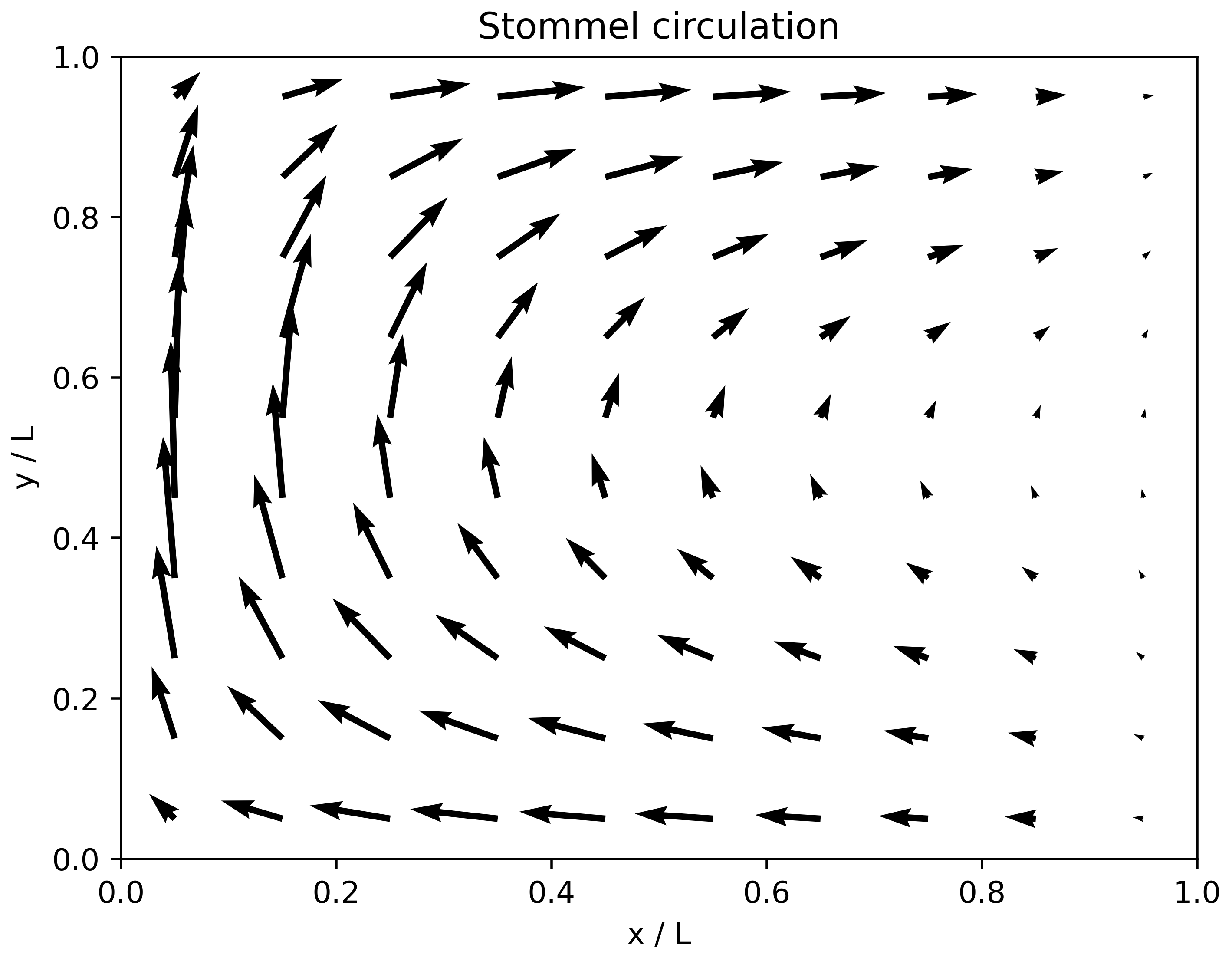
21.3.1.1 Stommel model

To parametrize the friction term at the bottom, one uses the Stommel model, which reads

\[ \begin{align} \mathbf{\tau}_B = r\newoverline{\mathbf{v}_{h}} \end{align} \]

with a constant $r > 0$. Since $w = 0$, we also have $\nabla\cdot \mathbf{v}_{h} = 0$, which is why the vertically averaged flow can be expressed in terms of a streamfunction $\psi$:

\[ \begin{align} \newoverline{u} = -\frac{\partial\psi}{\partial y}, & {} & \newoverline{v} = \frac{\partial\psi}{\partial x} \end{align} \]

Thus one can write

\[ \begin{align} \beta D\frac{\partial\psi}{\partial x} + \mathbf{k}\cdot\frac{1}{\rho_0}\nabla\times\mathbf{\tau}_B &= \mathbf{k}\cdot\frac{1}{\rho_0}\nabla\times\mathbf{\tau}_T\nonumber\\ \Leftrightarrow \beta D\frac{\partial\psi}{\partial x} + \frac{r}{\rho_0}\Delta\psi &= \mathbf{k}\cdot\frac{1}{\rho_0}\nabla\times\mathbf{\tau}_T\nonumber\\ \Leftrightarrow \frac{\partial\psi}{\partial x} + \frac{r}{\rho_0\beta D}\Delta\psi &= \frac{1}{\rho_0\beta D}\mathbf{k}\cdot\nabla\times\mathbf{\tau}_T\nonumber \end{align} \]

with

\[ \begin{align} \epsilon \coloneqq \frac{r}{\rho_0\beta D}. \end{align} \]

Eq. (21.14) is the equation of motion of the Stommel model. It applies Eq. (21.14) is the equation of motion of the Stommel model. One has

\[ \begin{align} \frac{\frac{\partial\psi}{\partial x}}{\epsilon\Delta\psi} \sim \frac{L\rho_0\beta D}{r} \end{align} \]

with $L$ as the horizontal length scale. For $r$, one estimates

\[ \begin{align} fV \sim \frac{Vr}{D\rho_0} \Rightarrow r \sim D\rho_0 f. \end{align} \]

Thus,

\[ \begin{align} \frac{\frac{\partial\psi}{\partial x}}{\epsilon\Delta\psi} \sim \frac{L \beta}{f} \sim \frac{L}{a}. \end{align} \]

As a rough approximation, for very large scales one may therefore work with

which represents another form of the Sverdrup balance. From this, the ocean current can be diagnosed for a given wind forcing.

Now Eq. (21.14) is solved on the set $\left[0, L\right] \times \left[0, L\right]$ with $L > 0$, i.e. for a square basin. This is only possible analytically in approximate form. One starts from a wind stress of the form

\[ \begin{align} \tau_T^{(x)} &= -\rho_0U^2\cos\left(\pi\frac{y}{L}\right),\\ \tau_T^{(y)} &= 0 \end{align} \]

From this it follows that

\[ \begin{align} \frac{\epsilon}{r}\mathbf{k}\cdot\nabla\times\mathbf{\tau}_T = -\frac{\epsilon\pi}{rL}\rho_0U^2\sin\left(\pi\frac{y}{L}\right). \end{align} \]

One makes the ansatz

\[ \begin{align} \psi = \psi_I + \phi, \end{align} \]

where $\psi_I$ is to approximate the solution in the interior of the basin and $\phi$ is to account for the boundary effects. In the interior of the basin, the larger scales are relevant, so the Sverdrup balance is assumed for $\psi_I$:

\[ \begin{align} \frac{\partial\psi_I}{\partial x} &= \frac{\epsilon}{r}\mathbf{k}\cdot\nabla\times\mathbf{\tau}_T = -\frac{\epsilon\pi}{rL}\rho_0U^2\sin\left(\pi\frac{y}{L}\right) \end{align} \]

This is solved by

\[ \begin{align} \psi_I = \left(C - x\right)\frac{\epsilon\pi}{rL}\rho_0U^2\sin\left(\pi\frac{y}{L}\right). \end{align} \]

with a constant $C$. The remaining part of the differential equation is to be solved by $\phi$:

\[ \begin{align} \epsilon\Delta\phi = 0 \end{align} \]

This is solved by

\[ \begin{align} \phi = -B\frac{\epsilon\pi}{rL}\rho_0U^2\sin\left(\pi\frac{y}{L}\right)\exp\left(\pm\pi\frac{x}{L}\right) \end{align} \]

with a constant $B$. The overall solution is therefore

\[ \begin{align} \psi = \psi_I + \phi = \left(C - x - B\exp\left(\pm\pi\frac{x}{L}\right)\right)\frac{\epsilon\pi}{rL}\rho_0U^2\sin\left(\pi\frac{y}{L}\right). \end{align} \]

This implies the following for the vertically averaged velocities:

\[ \begin{align} \newoverline{u} &= -\frac{\partial\psi}{\partial y} = -\frac{\pi}{L}\left(C - x - B\exp\left(\pm\pi\frac{x}{L}\right)\right)\frac{\epsilon\pi}{rL}\rho_0U^2\cos\left(\pi\frac{y}{L}\right),\tag{21.29}\label{eq:stommel_result_u}\\ \newoverline{v} &= \frac{\partial\psi}{\partial x} = \left(-1 \mp B\frac{\pi}{L}\exp\left(\pm\pi\frac{x}{L}\right)\right)\frac{\epsilon\pi}{rL}\rho_0U^2\sin\left(\pi\frac{y}{L}\right).\tag{21.30}\label{eq:stommel_result_v} \end{align} \]

$B$ and $C$ are determined from the boundary conditions. These are

\[ \begin{align} \newoverline{u}\left(x = 0, L\right) = 0, & {} & \newoverline{v}\left(y = 0, L\right) = 0. \end{align} \]

The boundary conditions for $\newoverline{v}$ are automatically satisfied. From those for $\newoverline{u}$ it follows that

\[ \begin{align} C = B, & {} & B - L - B\exp\left(-\pi\frac{L}{L}\right) = 0 \Rightarrow B = \frac{L}{1 - \exp\left(-\pi\right)}, \end{align} \]

where the negative sign in the exponential function has been chosen arbitrarily. This gives

21.3.1.2 Munk model

21.4 Thermohaline circulation

Thermohaline circulation describes the planetary circulation that arises because particles, as long as they are not subject to diabatic forcing, move along isopycnals. The basic idea is as follows:

1. Through diabatic fluxes, in particular evaporation and the resulting cooling and increase in salinity, the potential density of a water mass near the surface decreases.

2. The water mass sinks (deep-water formation), and the particles move along isopycnals through the ocean until the isopycnal reaches the surface again.

In practice, a large part of deep-water formation takes place in the North Atlantic after water transported there by the Gulf Stream has cooled through latent and sensible heat fluxes. This circulation is also known as the ocean conveyor belt. In the North Pacific, by contrast, no deep-water formation occurs because

• the trade winds transport freshwater in the form of precipitation from the Atlantic to the Pacific, so that the Atlantic is saltier, and

• water from the very salty Mediterranean reinforces deep-water formation in the Atlantic, which does not happen in the Pacific.

The water formed in the North Atlantic is called North Atlantic deep water (NADW). The densest and thus deepest water, however, is Antarctic bottom water (AABW). This water is not only very cold, but also very saline because ice formation expels salt, which gives it the highest potential density.

21.5 Ocean models

Ocean models simulate the state of the ocean, which is determined by the variables described in Section 21.1, analogous to atmospheric models, which simulate the state of the atmosphere. Compared to the atmosphere, ocean modeling has three major differences:

• The thermodynamic equation of state is considerably more complicated. In numerical terms, however, this is not a major problem.

• In the ocean there are no phase transitions. This is a major simplification, since it removes the need to compute phase transition rates and latent heat, and fewer tracers have to be advected.

• While the upper boundary of the atmosphere is set more or less arbitrarily, the water column has a clear vertical extent $[-H,\eta]$, where $H$ is the depth and $\eta$ is the displacement of the water surface due to currents (tides, wind-driven circulation, and waves). The difficulties here are that $H$ can become zero (land), and that $\eta$ is time dependent.

21.5.1 Prognostic variables

21.5.2 Vertical coordinates

Due to the challenge described in the previous section, the vertical coordinate plays a particularly important role in ocean modeling. In general, a vertical coordinate $\kappa$ is a bijective mapping

\[ \begin{align} z = z\left(\kappa\right). \end{align} \]

21.5.2.1 z-coordinates

With z-coordinates (also called geopotential coordinates), the coordinate surfaces are exactly horizontal. The main advantage is the absence of metric terms in horizontal derivatives. At the coasts, the coordinate surfaces intersect the ocean floor, so that the number of layers depends on the horizontal coordinates. Owing to the surface displacement $\eta$, the thickness of the first layer is moreover time dependent. The bathymetry is thereby represented in a step-like fashion.

21.5.2.2 $\sigma_z$-coordinates

With $\sigma_z$-coordinates, the layers are fitted to the bathymetry so that they do not intersect the ocean floor. In shallow waters the layers thereby become very thin, and on slopes the coordinate surfaces run very steeply. The mathematical formulation is analogous to the terrain-following coordinates in the atmosphere described in Section 12.3.

21.5.2.3 $\rho$-coordinates

Within the deeper ocean, the motions proceed predominantly along isopycnals. Aligning the coordinate surfaces with these is numerically advantageous, since vertical motions then almost vanish. This is, however, only possible if the ocean is stably stratified (otherwise the potential density within a water column cannot be mapped uniquely onto the geometric height), which is not the case everywhere, which is why these coordinates are not globally applicable. This is analogous to the isentropic coordinates in the atmosphere considered in Section 12.2.

21.5.2.4 $z^\star$-coordinates

$z^\star$-coordinates („z-star coordinates“) are a generalization of z-coordinates that resolves the problem that the thickness of the topmost layer depends on the surface displacement. The transformation to geometric coordinates reads

\[ \begin{align} z = \eta + z^\star\frac{\eta + H}{H}. \end{align} \]

The coordinate surfaces are therefore no longer exactly horizontal, but they still intersect the ocean floor.

21.5.2.5 Hybrid coordinates

All of the vertical coordinates listed so far have substantial advantages and disadvantages. Hybrid coordinates are an attempt to combine the advantages of the various coordinates with one another. Within the upper few tens of meters, the so-called thermocline, the ocean is well mixed and weakly stratified. Here, z- or $z^\star$-coordinates are appropriate. Further down, the ocean is dominated by quasi-geostrophic motions along the isopycnals (surfaces of equal potential density). In coastal regions, by contrast, terrain-following coordinates are appropriate in order to be able to represent the bathymetry. Hybrid coordinates are accordingly a mixture of $\rho-$, $\sigma_z-$, and $z^\star-$coordinates. They give the ocean model HyCOM (Hybrid Coordinate Ocean Model) its name.

21.6 Sea state forecast

21.6.1 Prognostic variables

Sea state is another word for water surface waves. The prognostic variable considered here is the displacement of the water surface

\[ \begin{align} h = h\left(x, y, t\right) \end{align} \]

from the mean position of the water surface.$h$ cannot simply be defined as a deviation from the geoid, since the dynamic topography would still be superimposed on it. This does not contribute to the displacement associated with the waves. The averaging interval must therefore be chosen accordingly. In many situations, $h$ is not a function of the horizontal coordinates, for example in surf or in a rough sea, because in such cases the position of the water surface is no longer uniquely defined. Such effects are accounted for later in the form of energy-dissipating source terms.

One could now use the shallow-water equations derived in Section 13.8.1 as a set of prognostic equations, possibly supplemented by some semi-empirical additional terms. However, this has several disadvantages:

• In order to capture a significant portion of the energy of the wave field, a very small time step and a very fine spatial resolution would be required.

• In most cases, the phases of the waves are not known and are not particularly relevant. Instead, quantities such as wave direction and wave height are decisive.

Therefore, water surface waves are usually described by means of a radiative transfer equation (RTE). The prognostic variable is then the spectral radiance

\[ \begin{align} N = N\left(\mathbf{k},\mathbf{r},t\right) \end{align} \]

Here $\mathbf{r}$ is a two-dimensional position vector and $\mathbf{k}$ is a two-dimensional wave vector. Usually, $\mathbf{k}$ is given not in Cartesian coordinates but in polar coordinates $\left(k,\theta\right)$. As the dispersion relation $\omega = \omega\left(k, \theta\right)$, one uses that of water surface waves

\[ \begin{align} \omega^2 &= gk\tanh\left(kD\right) \Rightarrow \omega = \sqrt{gk\tanh\left(kD\right)}, \end{align} \]

where $D$ is the mean water depth, i.e. the water depth without waves. From this it follows that

\[ \begin{align} c_\text{ph} &= \frac{\omega}{k} = \sqrt{\frac{g\tanh\left(kD\right)}{k}},\\ c_\text{gr} &= \frac{1}{2\omega}\frac{\partial\omega^2}{\partial k} = \frac{1}{2\omega}\left[g\tanh\left(kD\right) + \frac{gkD}{\cosh^2\left(kD\right)}\right] = \frac{g\tanh\left(kD\right)}{2\omega}\left[1 + \frac{kD}{\sinh\left(kD\right)\cosh\left(kD\right)}\right]\nonumber\\ &= \frac{c_\text{ph}}{2}\left[1 + \frac{2kD}{2\sinh\left(kD\right)\cosh\left(kD\right)}\right] = \frac{c_\text{ph}}{2}\left[1 + \frac{2kD}{\sinh\left(2kD\right)}\right]. \end{align} \]

Thus the group velocity is isotropic but not homogeneous,

\[ \begin{align} c_\text{gr} = c_\text{gr}\left(k,\mathbf{r},t\right). \end{align} \]

The spatial and temporal dependence arises through the spatial and temporal dependence of $D$.

21.6.2 Wave action equation

From this, one can derive a spectral radiative flux density

\[ \begin{align} N\left(k, \theta,\mathbf{r},t\right)\left(c_\text{gr}\left(k,\mathbf{r},t\right) + \mathbf{v}\left(\mathbf{r}, t\right)\right) \end{align} \]

where $\mathbf{v} = \mathbf{v}\left(\mathbf{r}, t\right)$ is the current velocity. The radiative transfer equation is a kind of continuity equation for $N$, which is conceptually related to the conservation of energy:

The spatial and temporal dependence is no longer written explicitly here. In addition, five source terms have been included:

• $S_\text{nl}\left(k, \theta\right)$ is the energy source resulting from nonlinear effects. This term is particularly relevant for interactions across scales. One example is the emergence of long waves, the so-called swell, from the shorter-wave wind sea produced directly by the wind, via upscaling.

• $S_\text{ws}\left(k, \theta\right)$ is the energy source resulting from interaction with the wind field. This is the main energy source of the wave field.

• $S_\text{wc}\left(k, \theta\right)$ is the energy source resulting from spray, the so-called whitecapping. This is a dissipative and therefore usually negative term.

• $S_\text{diss}\left(k, \theta\right)$ is the energy source associated with internal friction, i.e. viscosity. Since viscosity acts quadratically more strongly on the smaller scales, this effect causes wind sea to be dissipated faster than swell.

• $S_\text{bd}\left(k, \theta\right)$ is the energy source associated with interaction with the bathymetry, bottom drag. This, too, is a dissipative and therefore usually negative term.

Depending on the particular situation, further source terms can be included. Eq. (21.43) is also called the wave action equation.

The total energy of the wave spectrum $E$ at a given location and time is the integral over the entire spectrum:

\[ \begin{align} E = \int_0^{2\pi}\int_0^\infty N\left(k,\theta\right)dkd\theta.\tag{21.44}\label{eq:wave_spectrum_total_energy} \end{align} \]

The energy-weighted spectral mean of a quantity $\psi$ is therefore given by

\[ \begin{align} \newoverline{\psi} \coloneqq \frac{1}{E}\int_0^{2\pi}\int_0^\infty\psi\left(k,\theta\right)N\left(k,\theta\right)dkd\theta.\tag{21.45}\label{eq:wave_spectral_average} \end{align} \]

21.6.3 Diagnostic variables

21.6.3.1 Significant wave height

The significant wave height is a kind of representative wave height for which

\[ \begin{align} H_s = 4\sqrt{E}. \end{align} \]

21.6.3.2 Mean wave direction

The mean wave direction $\theta_m$ is calculated from Eq. (21.45) as

\[ \begin{align} \theta_m = \arctan2\left(b,a\right) \end{align} \]

with

\[ \begin{align} a &\coloneqq \frac{1}{E}\int_0^{2\pi}\int_0^\infty\cos\left(\theta\right)N\left(k,\theta\right)dkd\theta,\nonumber\\ b &\coloneqq \frac{1}{E}\int_0^{2\pi}\int_0^\infty\sin\left(\theta\right)N\left(k,\theta\right)dkd\theta. \end{align} \]

21.6.3.3 Mean wavelength

For the mean wavelength $L_m$, one has

\[ \begin{align} L_m = \newoverline{\left(\frac{2\pi}{k}\right)} = 2\pi\newoverline{k^{-1}}. \end{align} \]

21.6.3.4 Mean wave period

There are different ways of calculating the mean wave period:

\[ \begin{align} T_{m,1} &= \frac{2\pi}{\newoverline{\sigma}},\\ T_{m,2} &= \frac{2\pi}{\sqrt{\newoverline{\sigma^2}}},\\ T_{m,-1} &= \newoverline{\left(\frac{2\pi}{\sigma}\right)} = 2\pi\newoverline{\sigma^{-1}}. \end{align} \]

Here $\sigma$ is the angular frequency measured relative to the seabed.

21.6.4 Sea state forecast models

The most common sea-state forecast model is Wavewatch III. Models based on Eq. (21.43) are so-called third-generation sea-state forecast models. They solve this equation on a grid and are therefore grid-point models, even though they are sometimes referred to as spectral models because their prognostic variable has spectral meaning. They solve Eq. (21.43) by introducing, at each grid point, a spectral direction-dependent grid in $\left(k,\theta\right)$ space. In most cases, a fairly large variety of semi-empirical source terms $Q_i$ is also included.