22 Radiative transfer
The central quantity in radiative transfer is the spectral radiance $L_\kappa\left(\mathbf{r}, \mathbf{n}, t\right)$, where $\kappa$ is the wavenumber and $\mathbf{n}$ is a direction vector. From it, among other things, heat power densities can be derived.
22.1 Simple models
22.1.1 Planet without an atmosphere
The solar constant $S_0$ is the radiative flux density of the solar radiation reaching the Earth. Since the ratio of the surface to the cross-sectional area of a sphere is $4$, on average a radiative flux density $\frac{S_0}{4}$ is incident at the top of the atmosphere. Assuming that the Earth is a black body, in equilibrium the Stefan-Boltzmann law Eq. (5.326) yields
\[ \begin{align} \frac{S_0}{4} = \sigma T_\text{rad}^4, \end{align} \]
here $T_\text{rad}$ is the so-called radiation temperature. This can be extended by assuming a wavelength-independent emissivity $\epsilon$ and an albedo $\alpha \coloneqq 1 - \epsilon$:
\[ \begin{align} \frac{S_0}{4}\left(1 - \alpha\right) = \epsilon\sigma T_\text{rad}^4 \end{align} \]
Under the simplifying assumption that the long-wave (LW) and short-wave (SW) spectral ranges are separated from each other, one can use quantities $\epsilon_\text{SW}$, $\alpha_\text{SW}$, $\epsilon_\text{LW}$, $\alpha_\text{LW}$:
\[ \begin{align} \frac{S_0}{4}\left(1 - \alpha_\text{SW}\right) &= \epsilon_\text{LW}\sigma T_\text{rad}^4\nonumber\\ T_\text{rad} &= \left[\frac{S_0}{4\epsilon_\text{LW}\sigma}\left(1 - \alpha_\text{SW}\right)\right]^{1/4} \end{align} \]
Here one denotes
\[ \begin{align} \alpha_p \coloneqq \alpha_\text{SW} \end{align} \]
as the planetary albedo.
22.1.2 One-layer atmosphere
Now a homogeneous atmosphere, which consists of only a single layer, is included in the model. Atmospheric properties are denoted by the index $A$, while surface properties are denoted by the index $S$. Every subcomponent of the system (atmosphere, surface) is in thermal equilibrium. The applicable system of equations is therefore
\[ \begin{align} S_A^{(\text{in})} &= S_A^{(\text{out})} \Leftrightarrow S_{A, \text{SW}}^{(\text{in})} + S_{A, \text{LW}}^{(\text{in})} = S_{A, \text{SW}}^{(\text{out})} + S_{A, \text{LW}}^{(\text{out})},\tag{22.5}\label{eq:rad_atmos_single_layer_0}\\ S_S^{(\text{in})} &= S_S^{(\text{out})} \Leftrightarrow S_{S, \text{SW}}^{(\text{in})} + S_{S, \text{LW}}^{(\text{in})} = S_{S, \text{SW}}^{(\text{out})} + S_{S, \text{LW}}^{(\text{out})}.\tag{22.6}\label{eq:rad_atmos_single_layer_1} \end{align} \]
One now makes the following assumptions:
The atmosphere does not interact with short-wave radiation, so it transmits 100
The earth's surface reflects a portion $\alpha_{S, \text{SW}}$ of the short-wave radiation, the rest is absorbed. Since the reflected portion does not interact with the atmosphere, this energy propagates back into space.
The atmosphere is imagined as a single bar of homogeneous temperature that has a lower and an upper surface. In this model, the atmosphere has two surfaces from which it can emit long-wave radiation.
Within the short-wave or long-wave radiation range, the radiation properties are assumed to be independent of temperature and wavelength.
This results in the radiative flux densities
\[ \begin{align} S_{A, \text{SW}}^{(\text{in})} = 0,& {} & S_{A, \text{LW}}^{(\text{in})} = \epsilon_{A, \text{LW}}\epsilon_{S, \text{LW}}\sigma T_S^4,\\ S_{A, \text{SW}}^{(\text{out})} = 0,& {} & S_{A, \text{LW}}^{(\text{out})} = 2\epsilon_{A, \text{LW}}\sigma T_A^4,\\ S_{S, \text{SW}}^{(\text{in})} = \left(1 - \alpha_{S, \text{SW}}\right)\frac{S_0}{4},& {} & S_{S, \text{LW}}^{(\text{in})} = \epsilon_{A, \text{LW}}\sigma T_A^4,\\ S_{S, \text{SW}}^{(\text{out})} = 0,& {} & S_{S, \text{LW}}^{(\text{out})} = \epsilon_{S, \text{LW}}\sigma T_S^4. \end{align} \]
Substituting this into Eqs. (22.5) - (22.6), one obtains
\[ \begin{align} 0 + \epsilon_{A, \text{LW}}\epsilon_{S, \text{LW}}\sigma T_S^4 &= 0 + 2\epsilon_{A, \text{LW}}\sigma T_A^4,\\ \left(1 - \alpha_{S, \text{SW}}\right)\frac{S_0}{4} + \epsilon_{A, \text{LW}}\sigma T_A^4 &= 0 + \epsilon_{S, \text{LW}}\sigma T_S^4. \end{align} \]
Equivalent rearrangements yield
\[ \begin{align} T_A^4 &= \frac{\epsilon_{S, \text{LW}}}{2}T_S^4,\tag{22.13}\label{eq:rad_single_layer_deriv_0}\\ \epsilon_{S, \text{LW}}\sigma T_S^4 - \epsilon_{A, \text{LW}}\sigma T_A^4 &= \left(1 - \alpha_{S, \text{SW}}\right)\frac{S_0}{4}.\tag{22.14}\label{eq:rad_single_layer_deriv_1} \end{align} \]
Substituting Eq. (22.13) into Eq. (22.14), one obtains
\[ \begin{align} \epsilon_{S, \text{LW}}\sigma T_S^4 - \epsilon_{A, \text{LW}}\sigma\frac{\epsilon_{S, \text{LW}}}{2}T_S^4 &= \left(1 - \alpha_{S, \text{SW}}\right)\frac{S_0}{4}\nonumber\\ \Leftrightarrow\left(1 - \frac{\epsilon_{A, \text{LW}}}{2}\right)\epsilon_{S, \text{LW}}\sigma T_S^4 &= \left(1 - \alpha_{S, \text{SW}}\right)\frac{S_0}{4}\nonumber\\ \Leftrightarrow\left(1 - \frac{\epsilon_{A, \text{LW}}}{2}\right)T_S^4 &= \frac{S_0}{4\sigma\epsilon_{S, \text{LW}}}\left(1 - \alpha_{S, \text{SW}}\right)\nonumber\\ \Leftrightarrow T_S &= \left[\frac{S_0}{4\sigma\epsilon_{S, \text{LW}}\left(1 - \frac{\epsilon_{A, \text{LW}}}{2}\right)}\left(1 - \alpha_{S, \text{SW}}\right)\right]^{1/4} = T_\text{rad}\left(1 - \frac{\epsilon_{A, \text{LW}}}{2}\right)^{-1/4}. \end{align} \]
The inequality
\[ \begin{align} T_{S} > T_\text{rad} \end{align} \]
is called the greenhouse effect. This is based on the assumptions $\epsilon_{A, \text{LW}} > 0$ and $\alpha_{A, \text{SW}} = 0$. The simplest intuitive justification for the greenhouse effect is that the long-wave radiation is not emitted according to the temperature $T_S$, but according to the temperature $T_A < T_S$.
22.2 Feedbacks
Interactions between subsets of the Earth system are referred to as feedbacks. A distinction is made between positive feedback, which reinforces itself, and negative feedback, which dampens itself.
22.2.1 Temperature-radiation feedback
According to the Stefan-Boltzmann law, the radiation emitted by a body is proportional to the fourth power of the temperature. From this one obtains the following negative feedback:
Temperature rises $\rightarrow$ emission increases $\rightarrow$ temperature falls $\rightarrow$ emission decreases $\rightarrow$ temperature rises
Ultimately, this process describes the settling to a temperature at which the body under consideration is in equilibrium with the radiation field. Such considerations are always to be understood conceptually, which means that the oscillation suggested here does not necessarily have to take place.
22.2.2 Temperature-ice-albedo feedback
The planetary albedo $\alpha_p$ depends on the Earth's ice coverage: the higher the ice-covered portion, the more solar radiation is reflected. The feedback can be formulated conceptually in the form
Temperature increases $\rightarrow$ Ice melts $\rightarrow$ Planetary albedo decreases $\rightarrow$ more solar radiation is absorbed $\rightarrow$ Temperature increases
or, respectively,
Temperature drops $\rightarrow$ Water freezes $\rightarrow$ Planetary albedo increases $\rightarrow$ Less solar radiation is absorbed $\rightarrow$ Temperature drops
It is therefore a positive feedback.
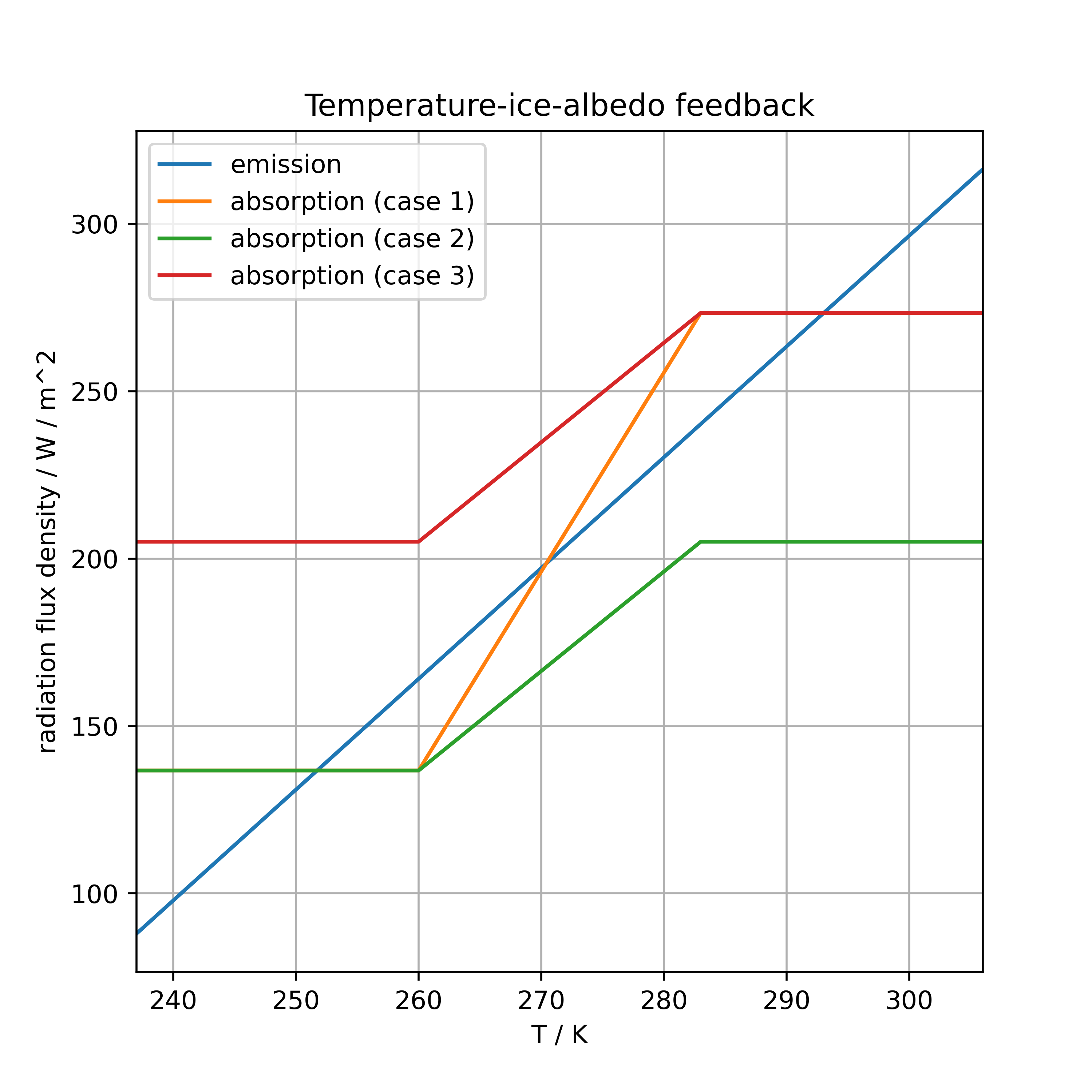
To quantify this, two temperatures $T_0 < T_1$ are introduced, and for the temperature-dependent planetary albedo one sets
\[ \begin{align} \alpha_p\left(T\right) = \begin{cases} \alpha_\text{max}, T < T_0\\ \alpha_\text{max} + \left(T - T_0\right)\frac{\alpha_\text{min} - \alpha_\text{max}}{T_1 - T_0}, T_0 \leq T \leq T_1\\ \alpha_\text{min}, T > T_1 \end{cases} \end{align} \]
with $0 \leq \alpha_\text{min} < \alpha_\text{max} \leq 1$. For the temperature-dependent emission $S = S\left(T\right)$ of the planet one further sets
\[ \begin{align} S\left(T\right) = a + b\left(T - \newoverline{T}\right) \end{align} \]
This corresponds to a linear expansion of the Stefan-Boltzmann law, so that
\[ \begin{align} a &= \sigma T_\text{rad}^4,\\ b &= 4\sigma T_\text{rad}^3. \end{align} \]
Here
\[ \begin{align} \newoverline{T} \coloneqq \frac{T_0 + T_1}{2} \end{align} \]
is the approximate temperature of the Earth, and
\[ \begin{align} T_\text{rad} \coloneqq 0,9\newoverline{T} \end{align} \]
a radiation temperature. In equilibrium one now has
\[ \begin{align} \frac{S_0}{4}\left(1 - \alpha_p\left(T\right)\right) &= a + b\left(T - \newoverline{T}\right). \end{align} \]
with the solar constant $S_0$. This equation has between one and three solutions depending on $T_0, T_1, \alpha_\mathrm{min}$ and $\alpha_\mathrm{max}$, as shown in Fig. 22.1. The equilibria in cases 2 and 3 are stable, while in case 1 the middle equilibrium is unstable and the outer two are stable.
22.3 Calculation of scattering and absorption coefficients
22.3.1 Effective radius
The effective radius is a size measure for condensates that well represents the properties they have in relation to their interaction with radiation. Assuming that all condensates are spherical and have radius $r_\text{eff}$, one obtains
\[ \begin{align} \frac{V}{A} = \frac{N\frac{4}{3}\pi r_\text{eff}^3}{N\pi r_\text{eff}^2} = \frac{4}{3}r_\text{eff}. \end{align} \]
Here $V$ is the total volume of the condensates, $A$ is their summed cross-sectional area (ignoring overlap) and $N$ is the number of condensates in the volume under consideration. From this it follows
\[ \begin{align} r_\text{eff} = \frac{3V}{4A}. \end{align} \]
The effective radius thus links the quantity $V$ (a bulk quantity), derivable from the mean density, with the cross-sectional area, which is the relevant quantity for the interaction with radiation.
22.4 Approximations
Apart from time, the spectral radiance depends on six real numbers. Ordinary fields depend on three coordinates. A first problem is accordingly the amount of storage space required to store even a very coarsely discretized radiation state of an atmosphere. Much more problematic, however, is the solution of the radiative transfer equation. Rigorous approximations are therefore necessary.
22.4.1 Plane-parallel atmosphere
This approximation assumes that the atmosphere within a certain region is horizontally homogeneous, so that the properties vary only vertically. This is motivated by the fact that in the atmosphere on large scales, horizontal gradients are at least two orders of magnitude smaller than vertical ones.
22.4.2 Horizontal decoupling
This approximation divides the atmosphere into independent columns and thereby greatly limits the horizontal interaction. However, such a column can consist of different sub-columns or horizontal interactions can be parameterized in another way within the columns. As computing capacity increases, the areas with horizontal interaction can be enlarged until, in the limit, the entire atmosphere is viewed as a single column.
22.5 Radiation balance
The radiation state of the atmosphere is completely described by the spectral radiance
\[ \begin{align} L = L\left(\mathbf{r}, \phi, \lambda, \omega, t\right). \end{align} \]
Many factors enter into the evolution of this quantity. The aim of this section is to quantify the importance of subcomponents of the climate system for the radiation field. This is called the radiation balance or also the radiation budget.