25 Basic concepts of numerics
A weather model is a copy of the atmosphere. In it, all fields and differential operators are replaced by discretized versions, since one can store only a finite amount of information. For a differential operator $D$, one writes a substitution
\[ \begin{align} D\to D', \end{align} \]
analogously for atmospheric states
\[ \begin{align} Z\to Z'. \end{align} \]
Next, one specifies a dynamics, i.e. a procedure
\[ \begin{align} Z'\left(t\right)\stackrel{D'}{\to}Z'\left(t + \Delta t\right) \end{align} \]
to determine the time evolution of the model atmosphere with the aim of bringing the state trajectory of the model as close as possible to that of the real atmosphere. To this end, one defines a distance
\[ \begin{align} \left|Z - Z'\right|\geq 0. \end{align} \]
Weather forecasting has the following workflow:
Observation of the state of the atmosphere.
Determination of the initial state of the model.
Integration of the model.
Errors arise for the following reasons:
The initial state was not fully observed.
The initial state was incorrectly observed.
The governing equations are equations of statistical physics and therefore do not apply exactly.
The model can store less information than the real atmosphere.
The dynamics of the model are different from those of the real atmosphere.
There are rounding errors due to the finite computer precision.
The computer makes errors.
25.1 Basic concepts of discretizations
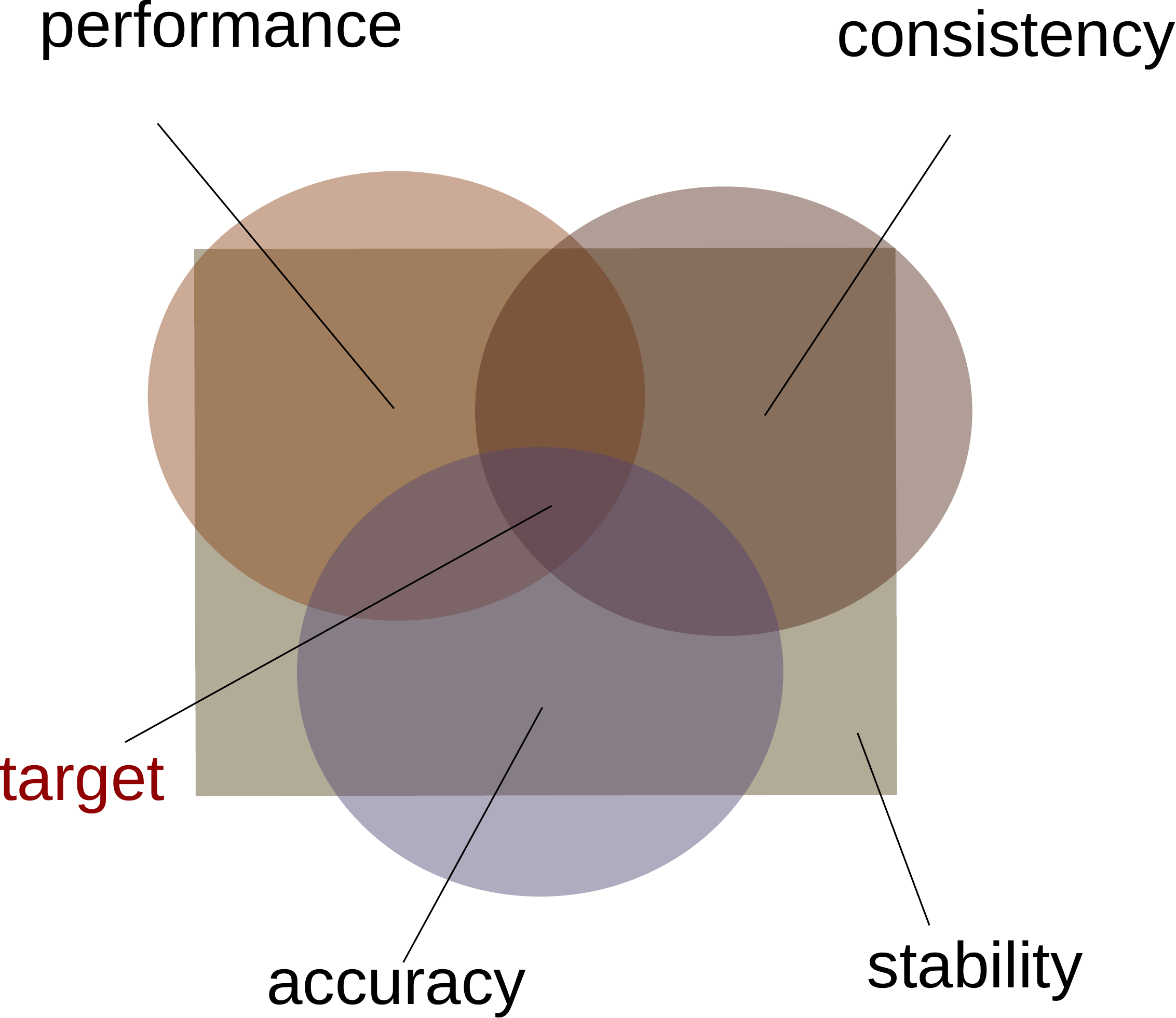
Let the solution of a differential equation be denoted by $F$ and the solution of a discretized version of the equation by $F_d$. A numerical procedure is called consistent if and only if the solution of the scheme converges to the solution of the differential equation as $\Delta x$ and $\Delta t$ become smaller, i.e. $\lim\limits_{\Delta\to 0}F_d = F$ in the above terms. A discretization is called self-consistent if all conserved quantities of the continuous system are also conserved quantities of the discretized system. This can also be transferred to approximations. A scheme is called stable if and only if the calculated solution is bounded for all times, i.e. if a $C>0$ exists with $|F_d|<C$ for all $t\geq t_0$ with $t_0$ as the starting time. Linear instability already arises with linear differential equations, whereas nonlinear instability can only arise with nonlinear differential equations.
25.2 Finite differences
Let $f:\mathbb{R}\to\mathbb{R}$ be an infinitely differentiable function. Using a Taylor series, one can write
\[ \begin{align} f\left(x + \Delta x\right) = f\left(x\right) + \Delta xf'\left(x\right) + \frac{f''\left(x\right)}{2!}\Delta x^2 + \frac{f'''\left(x\right)}{3!}\Delta x^3 + \dotsc\tag{25.5}\label{eq:taylor_links} \end{align} \]
and
\[ \begin{align} f\left(x - \Delta x\right) = f\left(x\right) - \Delta xf'\left(x\right) + \frac{f''\left(x\right)}{2!}\Delta x^2 - \frac{f'''\left(x\right)}{3!}\Delta x^3 + \dotsc\tag{25.6}\label{eq:taylor_rechts} \end{align} \]
Subtracting both equations yields
\[ \begin{align} f\left(x + \Delta x\right) - f\left(x - \Delta x\right) = 2\Delta xf'\left(x\right) + R', \end{align} \]
where the remainder $R'$ contains terms of third and higher order. Rearranging gives
\[ \begin{align} f'\left(x\right) = \frac{f\left(x + \Delta x\right) - f\left(x - \Delta x\right)}{2\Delta x} + R, \tag{25.8}\label{eq:approx_derivative_zentral} \end{align} \]
where $R$ is a polynomial in $\Delta x$ whose lowest power is 2; thus, Eq. (25.8) is a second-order approximation of the derivative, and one writes the symbol $\mathcal{O}\left(\Delta x^2\right)$ instead of $R$. This way of approximating derivatives is called a central difference quotient. A one-sided difference quotient, for example,
\[ \begin{align} f'\left(x\right) \approx\frac{f\left(x + \Delta x\right) - f\left(x\right)}{\Delta x} \end{align} \]
is also a suitable approximation, but it converges only to first order, as is easily seen by rearranging Eq. (25.5). The higher the order, the better, since the accuracy of a Taylor expansion increases with order. For this reason, central spatial difference quotients are used wherever possible. One can also derive an approximation for the second derivative of a function from Eqs. (25.5) and (25.6):
\[ \begin{align} f\left(x + \Delta x\right) + f\left(x - \Delta x\right)&= 2f\left(x\right) + f''\left(x\right)\Delta x^2 + \mathcal{O}\left(\Delta x^4\right)\nonumber\\ \Leftrightarrow f''\left(\Delta x\right) &= \frac{f\left(x + \Delta x\right) - 2f\left(x\right) + f\left(x - \Delta x\right)}{\Delta x^2} + \mathcal{O}\left(\Delta x^2\right) \end{align} \]
For example, for $f\left(x\right) = A\sin\left(kx\right)$ one has $f' = Ak\cos\left(kx\right)$, but Eq. (25.8) gives
\[ \begin{align} f' &\approx& \frac{A}{2\Delta x}\left(\sin\left(kx + k\Delta x\right) - \sin\left(kx - k\Delta x\right)\right) = \frac{A}{\Delta x}\cos\left(kx\right)\sin\left(k\Delta x\right) = \frac{\sin\left(k\Delta x\right)}{k\Delta x}f'. \end{align} \]
This shows that the approximation converges, as expected, to the correct derivative as $\Delta x$ approaches zero (since $\lim\limits_{\alpha\to 0}\frac{\sin\left(\alpha\right)}{\alpha} = 1$ by L'Hospital's rule). Writing $k = \frac{2\pi}{\lambda}$ with $\lambda$ as wavelength and setting $\Delta x = \lambda/2$, the central difference quotient always yields $f' = 0$. However, sufficiently long waves ($\lambda\gg 2\Delta x$) are well resolved.
25.3 Plane spectral method
The plane spectral method rests on Fourier-transforming the horizontal dependencies of the state variables. This transformation is set out in Sect. C.1. The quantities $x,y$ may be any horizontal coordinates, such as geographic longitude and latitude, the spherical coordinates of a rotated longitude-latitude grid, or coordinates defined within a map projection such as the Lambert projection. A well-known dynamical core that employs this method is ALADIN, which underlies the models AROME and HARMONIE.
25.4 Spherical spectral method
Let $\psi = \psi\left(\varphi, \lambda, z\right)$ be a scalar field. Since the spherical harmonics presented in Sect. C.5 form a complete orthonormal basis on spherical shells, the horizontal dependence of $\psi$ can be represented by this set of functions:
\[ \begin{align} \psi\left(\varphi, \lambda, z\right) = \sum_{l = 0}^\infty\sum_{m = -l}^l\newtilde{\psi}_{l, m}\left(z\right)Y_{l, m}\left(\varphi, \lambda\right) \end{align} \]
The definition of the spherical harmonics, Eq. (C.155), is written here in geographic coordinates:
\[ \begin{align} Y_{l, m}\left(\varphi, \lambda\right) = \sqrt{\frac{2l + 1}{4\pi}\frac{\left(l - m\right)!}{\left(l + m\right)!}}P_{l, m}\left(\sin\left(\varphi\right)\right)\exp\left(im\lambda\right) \end{align} \]
25.5 Parameterizations
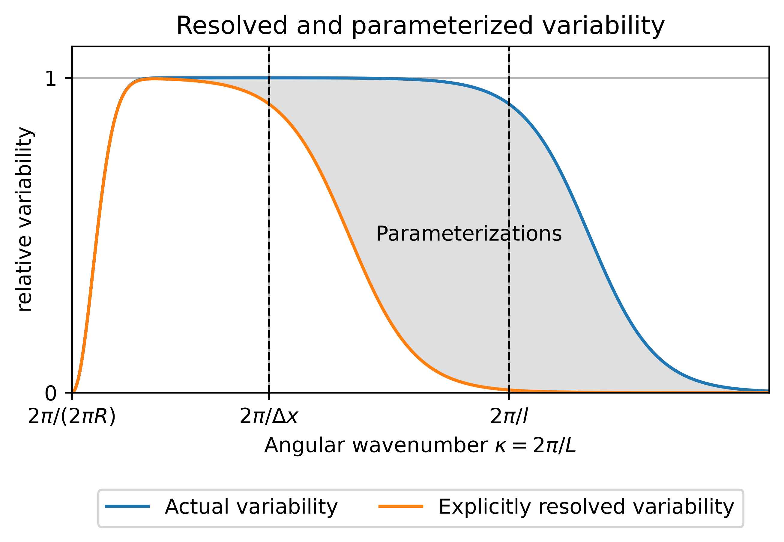
Estimating the effects of subscale variability on the averaged variables is called parameterization. This is illustrated in Fig. 25.2. At first, one might assume that the subscale variability can simply be ignored, precisely because it is not resolved by the chosen discretization. This would indeed be the case for a linear system of differential equations, since in linear systems of differential equations the different scales do not interact with each other. The only problem of a coarse resolution would then be that the exact values of the prognostic variables at a given location and time are unknown. In particular, in the linear case there would be no exponential growth of the model error with time. In nonlinear systems of equations, however, the scales do interact with each other, so that the unresolved scales influence the resolved ones. Since reducing the grid spacing in numerical models is very expensive, the unresolved variability is parameterized by numerical approaches (in the simplest case merely an algebraic formula added to a prognostic equation), which are orders of magnitude cheaper to compute than an explicit simulation.
Fig. 25.2 illustrates an important principle that should be kept in mind when developing parameterizations and configuring models: variability at a given angular wavenumber $k$ should always be represented correctly in the model, either by the explicit simulation (i.e., the resolved part) or by the parameterizations. The following three errors occur frequently in this context:
The variability is underrepresented: it is fully captured neither explicitly nor by the parameterizations.
The variability is both simulated explicitly and parameterized, and is therefore overrepresented.
The variability is captured by two different parameterizations, and is therefore likewise overrepresented.
Difficulties always arise in the spectral transition region between the explicitly resolved part and the parameterizations, or between two parameterizations. The ability of a parameterization to adapt to different model resolutions is referred to as scale awareness. If all parameterizations in a model are scale-aware, the model can be run with resolution-independent settings. Many parameterizations, however, do not satisfy this criterion, because they were developed for models of a certain resolution. This does not mean that the parameterization is unphysical or inaccurate; it merely must not be used outside the resolution range for which it was developed.
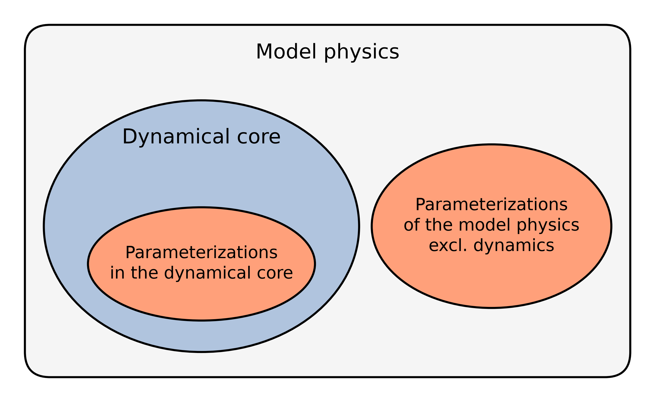
Unfortunately, the term parameterization is frequently equated with the term „physics“, where physics here refers to aspects such as radiation and cloud physics, in contrast to „dynamics“, which refers to hydrodynamics. The justification is often that processes such as radiation and cloud physics take place on the molecular scale, i.e., on scales not resolved by the model, which supposedly makes parameterization necessary. This is inconsistent, however: the pressure gradient also builds up on the molecular scale via collisions between particles, yet it is simulated by the dynamical core. In truth, both the dynamics and the physics of the model (in the sense explained above) have resolved and unresolved parts, and it is the unresolved parts that are parameterized. A radiative transfer algorithm, for instance, is not a parameterization but a simulation of a physical process, just as the dynamical core simulates another physical process. The same applies to cloud physics, the soil simulation, or other components. If, however, the radiative fluxes are modified by assuming clouds that are not explicitly resolved by the model, this does constitute a parameterization.
25.5.1 Scalar advection
Nature diffuses the quantities temperature $T$ and gas densities $\rho_i$. Let $\psi$ be such a quantity. The diffusion occurs through a diffusion coefficient $\kappa_\psi$ that depends on the thermodynamic state variables and therefore depends on location and time. One writes
\[ \begin{align} \frac{\partial\psi}{\partial t} = \dots + \nabla\cdot\left(\kappa_\psi\nabla\psi\right). \end{align} \]
$\kappa_{\psi}$ is first of all of molecular origin. The covariance terms of scalar advection $-\newoverline{\mathbf{v}''\cdot\nabla\psi''}$ that arise when averaging nonlinear systems are sensibly parameterized by making the ansatz
\[ \begin{align} \kappa_{\psi, \Delta} = \kappa_\psi + \kappa_{\psi, S},\tag{25.15}\label{eq:para_ansatz_0} \end{align} \]
where the index $\Delta$ represents the diffusion coefficient to be used in the discretization and the index $S$ represents the effect of the subscale. In this way, physical self-consistency is guaranteed. As $\Delta x, \Delta t$ become smaller, i.e. with higher resolution, $\kappa_{\psi, \Delta}$ converges to $\kappa_{\psi}.$ At low resolution, a good approximation is $\kappa_{\psi, \Delta} = \kappa_{\psi, S}$. Since the vertical grid point spacing is usually significantly smaller than the horizontal one, $\kappa_{\psi, S}$ can be assumed to be direction-dependent, i.e.
\[ \begin{align} \kappa_{\psi, \Delta}\nabla\psi \to \kappa_{\psi, \Delta, H}\nabla_h\psi + \kappa_{\psi, \Delta, z}\frac{\partial\psi}{\partial z}\mathbf{k}. \end{align} \]
Here the horizontal diffusion coefficient is greater than the vertical one.
25.5.2 Momentum advection
In order to derive an ansatz for the parameterization of momentum advection, one proceeds analogously to the case of scalar advection in the previous section, starting from the ansatz that the subscale variability leads to an isotropic diffusion. This also corresponds to the mixing-length approach described in Sect. 17.2. There it was assumed that the fluid transports its properties unchanged over a certain length, the so-called mixing length, before it equilibrates with its surroundings. This is also the case with molecular diffusion, and thus also with friction as a special case. One first recalls Eq. (8.52) for the frictional acceleration $\mathbf{f}_R$:
\[ \begin{align} \mathbf{f}_R &= \nu\Delta\mathbf{v} + \left(\frac{\mu_v}{\rho} + \frac{\nu}{3}\right)\nabla\left(\nabla\cdot\mathbf{v}\right) \stackrel{\href{ch-39-vector-analysis.html#eq:diff_op_rule_8}{\text{Eq. (B.54)}}}{=} \left(\frac{\mu_v}{\rho} + \frac{4\nu}{3}\right)\nabla\left(\nabla\cdot\mathbf{v}\right) - \nu\nabla\times\left(\nabla\times\mathbf{v}\right)\nonumber\\ &= \left(\frac{\mu_v}{\rho} + \frac{4\nu}{3}\right)\nabla D - \nu\nabla\times\zetabi \end{align} \]
The following analogy can be used as a modified justification for this ansatz: The Maxwell distribution Eq. (5.191) is isotropic. Atoms and molecules are subscale within the Navier-Stokes equations. Their isotropic momentum distribution is superimposed on the wind velocity $\mathbf{v}$. This has the physical effect of the existence of the frictional acceleration Eq. (8.52) and the dissipation Eq. (8.66). If the turbulent (subscale) motion is isotropic, one can assume that the turbulence has similar effects on the averaged quantities. This analogy also holds for the diffusive ansätze for the subscale transport of scalar quantities.
However, the effective viscosities remain to be determined. In a discretization, one now sets, analogously to Eq. (25.15),
\[ \begin{align} K = \nu + \nu_S,& {} & K_v = \mu_v + \mu_{v, S} \end{align} \]
From this it follows for the effective frictional acceleration
\[ \begin{align} \mathbf{f}_R &= \left(\frac{K_v}{\rho} + \frac{4K}{3}\right)\nabla D - K\nabla\times\zetabi.\tag{25.19}\label{eq:friction_acceleration_for_discrete} \end{align} \]
25.5.3 Phase transitions
Let $\rho_v$ be the density of water vapor, the advection equation for this quantity is
\[ \begin{align} \frac{\partial\rho_v}{\partial t} = -\nabla\cdot\left(\rho_v\mathbf{v}\right) + s_v, \end{align} \]
here $s_v$ is the source density of the water vapor. Integrating this equation over a set $\Omega \subseteq \mathbb{R}^3$, one obtains, using Gauss's theorem,
\[ \begin{align} \int_\Omega\frac{\partial\rho_v}{\partial t}d^3r = -\int_\Omega\nabla\cdot\left(\rho_v\mathbf{v}\right)d^3r = -\int_{\partial\Omega}\rho_v\mathbf{v}\cdot d\mathbf{n} + \int_\Omega s_vd^3rdt'. \end{align} \]
If one further integrates over a time interval $\left[t, t + \Delta t\right]$, it follows
\[ \begin{align} \int_t^{t + \Delta t}\int_\Omega\frac{\partial\rho_v}{\partial t}d^3rdt' &= -\int_t^{t + \Delta t}\int_{\partial\Omega}\rho_v\mathbf{v}\cdot d\mathbf{n}dt' + \int_t^{t + \Delta t}\int_\Omega s_vd^3rdt'\nonumber\\ \Leftrightarrow\int_\Omega\rho_v\left(t + \Delta t\right) - \rho_v\left(t\right)d^3r &= -\int_t^{t + \Delta t}\int_{\partial\Omega}\rho_v\mathbf{v}\cdot d\mathbf{n}dt' + \int_t^{t + \Delta t}\int_\Omega s_vd^3rdt'\nonumber\\ \Leftrightarrow V\left[\newoverline{\rho_v}\left(t + \Delta t\right) - \newoverline{\rho_v}\left(t\right)\right] &= -\int_t^{t + \Delta t}\int_{\partial\Omega}\rho_v\mathbf{v}\cdot d\mathbf{n}dt' + \int_t^{t + \Delta t}\int_\Omega s_vd^3rdt'\nonumber\\ \Leftrightarrow \newoverline{\rho_v}\left(t + \Delta t\right) &= \newoverline{\rho_v}\left(t\right) - \frac{1}{V}\int_t^{t + \Delta t}\int_{\partial\Omega}\rho_v\mathbf{v}\cdot d\mathbf{n}dt' + \int_t^{t + \Delta t}\int_\Omega s_vd^3rdt'\nonumber\\ \Leftrightarrow \newoverline{\rho_v}\left(t + \Delta t\right) &= \newoverline{\rho_v}\left(t\right) - \frac{1}{V}\int_t^{t + \Delta t}\int_{\partial\Omega}\rho_v\mathbf{v}\cdot d\mathbf{n}dt' + \int_\Omega\int_t^{t + \Delta t}s_vdt'd^3r.\tag{25.22}\label{eq:phase_trans_para_deriv_0} \end{align} \]
For the sake of simplicity, it is assumed at this point that there are no condensates at time $t$ and that no phase transitions in the direction of water vapor take place during the time interval $\left[t, t + \Delta t\right]$. In this case, one has
\[ \begin{align} \int_t^{t + \Delta t}s_vdt' = -\Theta\left[\rho_v\left(t + \Delta t\right) - \rho_v^{(\text{sat})}\left(t + \Delta t\right)\right]\left[\rho_v\left(t + \Delta t\right) - \rho_v^{(\text{sat})}\left(t + \Delta t\right)\right] \leq 0. \end{align} \]
One thus has
\[ \begin{align} Q_v \coloneqq \int_\Omega\int_t^{t + \Delta t}s_vdt'd^3r = -\int_\Omega\Theta\left[\rho_v\left(t + \Delta t\right) - \rho_v^{(\text{sat})}\left(t + \Delta t\right)\right]\left[\rho_v\left(t + \Delta t\right) - \rho_v^{(\text{sat})}\left(t + \Delta t\right)\right]d^3r \leq 0. \end{align} \]
Now define
\[ \begin{align} \newtilde{Q}_v &\coloneqq -\Theta\left\{\newoverline{\rho_v}\left(t + \Delta t\right) - \rho_v^{(\text{sat})}\left[\newoverline{T}\left(t + \Delta t\right), \newoverline{p}\left(t + \Delta t\right)\right]\right\}\left\{\rho_v\left(t + \Delta t\right) - \rho_v^{(\text{sat})}\left[\newoverline{T}\left(t + \Delta t\right), \newoverline{p}\left(t + \Delta t\right)\right]\right\} \leq 0\nonumber\\ & \end{align} \]
This is the source term that would result if the phase transition were calculated from the averaged thermodynamic quantities (in a model these would be the values in the grid boxes). One has
\[ \begin{align} Q_v \leq \newtilde{Q}_v. \end{align} \]
Now define the difference between the actual phase transition and the one computed from the averaged quantities by
\[ \begin{align} \Delta Q_v \coloneqq Q_v - \newtilde{Q}_v \leq 0. \end{align} \]
This allows Eq. (25.22) to be written in the form
\[ \begin{align} \newoverline{\rho_v}\left(t + \Delta t\right) &= \newoverline{\rho_v}\left(t\right) - \frac{1}{V}\int_t^{t + \Delta t}\int_{\partial\Omega}\rho_v\mathbf{v}\cdot d\mathbf{n}dt' + Q_v\nonumber\\ &= \newoverline{\rho_v}\left(t\right) - \frac{1}{V}\int_t^{t + \Delta t}\int_{\partial\Omega}\rho_v\mathbf{v}\cdot d\mathbf{n}dt' + \newtilde{Q}_v + \Delta Q_v. \end{align} \]
The source term $Q_v$ is therefore composed of two parts:
The term $\newtilde{Q}_v \leq 0$ corresponds to the resolved part.
The term $\Delta Q_v \leq 0$ corresponds to the subscale part.
A model would initially only have knowledge of the resolved portion $\newtilde{Q}_v$ and would therefore underestimate the overall phase transition $Q_v$. In particular, there can be situations with $\newtilde{Q}_v = 0$ and $\Delta Q_v < 0$. One can now derive ansätze for the term $\Delta Q_v$ from derived or measured spectral properties of the fields.
This section further illustrates that all types of parameterizations ultimately have to do with subscale variability. In the case $\Omega, \Delta t \to 0$, $\Delta Q_v$ approaches zero, which is also the case for all parameterizations.
25.5.4 Convection
Convection occurs locally in the presence of thermal instability, i.e. in the case
\[ \begin{align} N^2 < 0.\tag{25.29}\label{eq:conv_crit_local} \end{align} \]
However, if one averages over a base area $A\subseteq\mathbb{R}^2$, then, owing to the variability of $N$, i.e.
\[ \begin{align} N^2_\text{min}\leq\newoverline{N^2}, \end{align} \]
Eq. (25.29) is locally satisfied somewhere within $A$ before the criterion is satisfied on average.
25.5.5 Tuning
Parameterizations approximate complex subgrid-scale effects by simplified ansatzes. The general form of these ansatzes is usually derived from theory under simplifying assumptions. Owing to these assumptions, the resulting formulas are not exact. In order to increase the accuracy nevertheless, one can modify the coefficients appearing in the parameterizations. Two methods lend themselves to this purpose:
They can be inferred from measurements.
They can be inferred from DNS runs (direct numerical simulation), i.e. very high-resolution simulations in the computational fluid dynamics (CFD) regime.
This yields plausible intervals within which the coefficients to be determined can be chosen freely. Within these intervals, one then chooses them such that the model is as accurate as possible. Since several parameters can be tuned in an atmospheric model, this formally becomes a multidimensional optimization problem requiring many iterations, each of which involves many model runs. To limit the number of dimensions of this optimization problem, one does not always fit all coefficients to be tuned with respect to the overall accuracy of the model; instead, one reduces the number of degrees of freedom by expressing certain coefficients in terms of others, or one optimizes only with respect to a specific partial aspect that can be examined without having to perform complete model runs.