25 Time step method

Let $\psi: A \subseteq \mathbb{R}^3 \times \mathbb{R} \to \mathbb{R}^n$ be the atmospheric state vector. All fundamental physical laws are first order in time, therefore one can write

\[ \begin{align} \frac{d\psi}{dt} = F\left(\psi\right), \end{align} \]

where $F$ contains the physics. If you discretize this onto a temporal grid $n\Delta t$ with $n \in \mathbb{Z}$ and interpolate between two time steps $n$, $n + l$, you get

\[ \begin{align} \psi_{n + l} - \psi_{n} = \int_{n\Delta t}^{\left(n + l\right)\Delta t}F\left(\psi\right)dt. \end{align} \]

The number of time steps involved is $l + 1$. You can now discretize the integral on the right-hand side in a variety of ways. The explicit Euler method results from the approximation with $l = 1$

\[ \begin{align} \int_{n\Delta t}^{\left(n + 1\right)\Delta t}F\left(\psi\right)dt \approx F\left(\psi_{n}\right)\Delta t \end{align} \]

with $\psi_{n} \coloneqq \psi\left(n\Delta t\right)$. The implicit Euler method, on the other hand, is obtained via

\[ \begin{align} \int_{n\Delta t}^{\left(n + 1\right)\Delta t}F\left(\psi\right)dt \approx F\left(\psi_{n + 1}\right)\Delta t \end{align} \]

This chapter aims to explain how the time discretization of a linear differential equation can affect the dispersion relation and the stability of a wave solution. It becomes the linear advection equation

\[ \begin{align} \frac{\partial f}{\partial t} + U\frac{\partial f}{\partial x} = 0\tag{25.5}\label{eq:test_lineare_instab} \end{align} \]

considered with $U\not = 0$ as a homogeneous advection velocity and $f$ as some particle property. The analytical solution is in the complex notation

\[ \begin{align} f = \exp\left(i\left(kx - \omega t\right)\right), \end{align} \]

If you insert this, $-i\omega + Uik = 0$, i.e. as a dispersion relation

\[ \begin{align} \omega = Uk. \end{align} \]

So phase and group speed are equal to $U$. Now place and time are discretized, you write $f_l^{(m)} = f\left(l\Delta x, m\Delta t\right)$ and start

\[ \begin{align} f_{l}^{(m)} = e^{Cm\Delta t}e^{i\left(kl\Delta x - \omega m\Delta t\right)}\tag{25.8}\label{eq:ansatz_time_stepping_1d_analysis} \end{align} \]

with $f_{l}^{(0)} = e^{ikl\Delta x}$ as the initial state. Here $C$, $k$ and $\omega$ are real numbers. For reasons of symmetry, $k$ cannot have an imaginary part. $C$ and the dispersion $\omega\left(k\right)$ are to be determined.

25.1 Purely explicit procedures

25.1.1 Explicit Euler method

First, the following discretization is examined:

\[ \begin{align} \frac{f_l^{(m + 1)} - f_l^{(m)}}{\Delta t} + U\frac{f_{l + 1}^{(m)} - f_{l - 1}^{(m)}}{2\Delta x} = 0 \end{align} \]

This is called explicit Euler method. insertion results in

\[ \begin{align} \frac{e^{C\Delta t}e^{-i\omega\Delta t} - 1}{\Delta t} + U \frac{e^{ik\Delta x} - e^{-ik\Delta x}}{2\Delta x} = \frac{e^{C\Delta t}\cos\left(\omega\Delta t\right) - ie^{C\Delta t}\sin\left(\omega\Delta t\right) - 1}{\Delta t} + \frac{iU\sin\left( k\Delta x\right)}{\Delta x} = 0. \end{align} \]

The real part is

\[ \begin{align} e^{C\Delta t}\cos\left(\omega\Delta t\right) = 1, \end{align} \]

from this it follows i. A. $C> 0$, there is instability. This is linear instability, since Eq. (25.5) is linear in $f$. The imaginary part is

\[ \begin{align} e^{C\Delta t}\sin\left(\omega\Delta t\right) = \frac{U\Delta t\sin\left(k\Delta x\right)}{\Delta x}. \end{align} \]

From this it follows

\[ \begin{align} \tan\left(\omega\Delta t\right) = \frac{U\Delta t\sin\left(k\Delta x\right)}{\Delta x}, \end{align} \]

so the dispersion

\[ \begin{align} \omega\left(k\right) = \frac{1}{\Delta t}\arctan\left(\frac{U\Delta t\sin\left(k\Delta x\right)}{\Delta x}\right). \end{align} \]

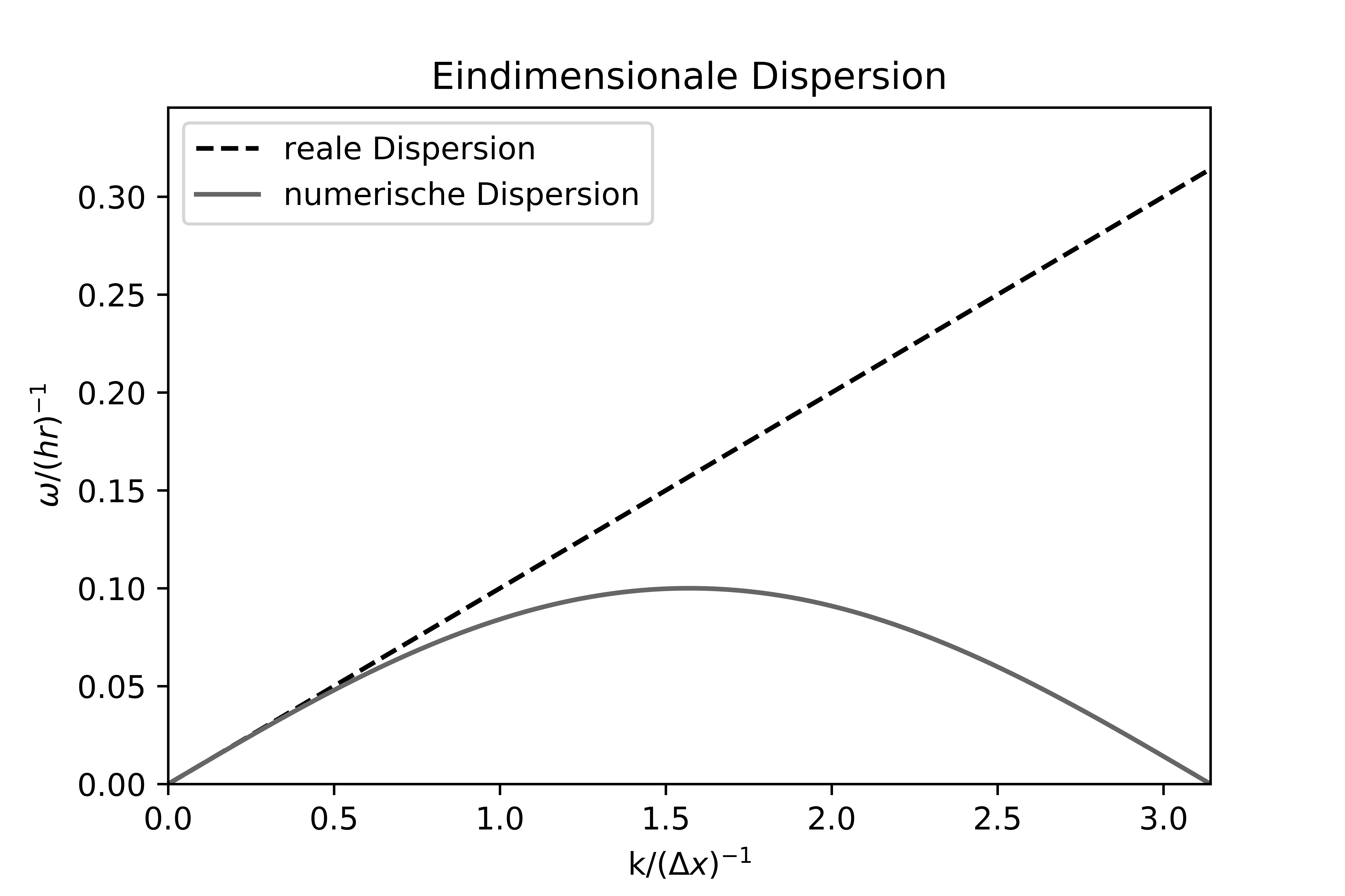
Let $\lambda$ be the wavelength, i.e. $k = \frac{2\pi}{\lambda}$. For $\lambda\gg \Delta x$ we have $\sin\left(k\Delta x\right) \approx k\Delta x$, i.e. $\omega \approx \frac{1}{\Delta t}\arctan\left(Uk\Delta t\right)$. In the case $U\Delta t\ll \lambda$, i.e. $Uk\Delta t\ll 1$, $\omega \approx \frac{1}{\Delta t}U\Delta t k = Uk$ as in the continuous case. Long waves are resolved well with a sufficiently small time step. However, for the shortest resolved wave $\lambda = 2\Delta x$ it follows $\omega = \frac{1}{\Delta t}\arctan\left(\frac{U\Delta t\sin\pi}{\Delta x}\right) = 0$, so the wave is stationary. Fig. 25.1 shows the dispersion relation for the case $U = 10$ m/s. You can see that waves with $k\leq \frac{1}{\Delta x}$, i.e. $\lambda\geq 2\pi\Delta x$, are simulated decently.

25.1.1.1 First-order upwind procedure

In the case $U>0$ it is called discretization

\[ \begin{align} \frac{f_l^{(m + 1)} - f_l^{(m)}}{\Delta t} + U\frac{f_{l}^{(m)} - f_{l - 1}^{(m)}}{\Delta x} = 0 \end{align} \]

as first-order-upwind method. This leads to

\[ \begin{align} \frac{e^{C\Delta t}e^{-i\omega\Delta t} - 1}{\Delta t} + U \frac{1 - e^{-ik\Delta x}}{\Delta x} = \frac{e^{C\Delta t}\cos\left(\omega\Delta t\right) - ie^{C\Delta t}\sin\left(\omega\Delta t\right) - 1}{\Delta t} + U\frac{1 - \cos\left( k\Delta x\right) + i\sin\left(k\Delta x\right)}{\Delta x} = 0. \end{align} \]

The imaginary part of this is

\[ \begin{align} &\frac{e^{C\Delta t}\sin\left(\omega\Delta t\right)}{\Delta t} = U\frac{\sin\left(k\Delta x\right)}{\Delta x}\nonumber\\ &\Leftrightarrow e^{C\Delta t}\sin\left(\omega\Delta t\right) = U\frac{\Delta t\sin\left(k\Delta x\right)}{\Delta x}\nonumber\\ &\Leftrightarrow e^{C\Delta t} = U\frac{\Delta t\sin\left(k\Delta x\right)}{\Delta x\sin\left(\omega\Delta t\right)}. \end{align} \]

The discretization is stable if and only if $C\leq 0$, i.e. for

\[ \begin{align} U\frac{\Delta t\sin\left(k\Delta x\right)}{\Delta x\sin\left(\omega\Delta t\right)}\leq 1. \end{align} \]

Because of

\[ \begin{align} c = \frac{\omega}{k}\leq\frac{\Delta x}{\Delta t}\Leftrightarrow\omega\Delta t\leq k\Delta x \end{align} \]

the estimate continues

This equation is called Courant-Friedrichs-Lewy criterion (CFL criterion). One defines the Courant number or CFL number $c$ by

\[ \begin{align} c\coloneqq\frac{U\Delta t}{\Delta x}. \end{align} \]

The CFL criterion is linguistic

25.1.2 Leapfrog procedure

If you use a central temporal difference quotient, write:

\[ \begin{align} \frac{f_l^{(m + 2)} - f_l^{(m)}}{2\Delta t} + U\frac{f_{l + 1}^{(m + 1)} - f_{l - 1}^{(m + 1)}}{2\Delta x} = 0, \end{align} \]

so this results in used

\[ \begin{align} \frac{e^{2C\Delta t}e^{-2i\omega\Delta t} - 1}{2\Delta t} + U \frac{e^{ik\Delta x}e^{C\Delta t}e^{-i\omega\Delta t} - e^{-ik\Delta x}e^{C\Delta t}e^{-i\omega\Delta t}}{2\Delta x} &= 0 \nonumber\\ \Leftrightarrow \frac{e^{C\Delta t}e^{-i\omega\Delta t} - e^{-C\Delta t}e^{i\omega\Delta t}}{2\Delta t} + U \frac{e^{ik\Delta x} - e^{-ik\Delta x}}{2\Delta x} &= 0. \end{align} \]

The real part results

\[ \begin{align} e^{C\Delta t}\cos\left(\omega\Delta t\right) = e^{-C\Delta t}\cos\left(\omega\Delta t\right). \end{align} \]

This means $C = 0$, so the solution is stable. The imaginary part becomes

\[ \begin{align} \frac{\sin\left(\omega\Delta t\right)}{2\Delta t}\left(e^{-C\Delta t} + e^{C\Delta t}\right) = \frac{\sin\left(\omega\Delta t\right)}{\Delta t} = U\frac{\sin\left(k\Delta x\right)}{\Delta x}. \end{align} \]

It follows

\[ \begin{align} \sin\left(\omega\Delta t\right) = U\frac{\Delta t}{\Delta x}\sin\left(k\Delta x\right)\Rightarrow\omega = \frac{1}{\Delta t}\arcsin\left[\frac{U\Delta t}{\Delta x}\sin\left(k\Delta x\right)\right], \end{align} \]

i.e. a different dispersion relation than in the explicit case. In general, the stability of the solution seems to follow from the real part, while the dispersion seems to follow from the imaginary part. Schemes are still either stable ($C \leq 0$), labile ($C > 0$) or conditionally stable (stable for sufficiently small $\Delta t$). This is influenced by the time step method. The optimal case is $C = 0$, which results from the leapfrog method, so this method is the most suitable.

25.1.3 General multistep procedures

25.1.4 Runge-Kutta method

Let $f: \mathbb{R}^l\times\mathbb{R} \to \mathbb{R}^m$ with $l, m \geq 1$ be an infinitely often continuously differentiable function, which solves the initial value problem

\[ \begin{align} \frac{df}{dt} = F\left[f\left(t\right)\right], & {} & f_0 = f_0 \end{align} \]

fulfilled. So-called Runge-Kutta procedures are based on calculating several values ​​for $df/dt$ and superimposing them in such a way that as many terms of the Taylor series as possible are covered.

25.1.4.1 Linear case

The Taylor expansion of $f$ is

\[ \begin{align} f\left(t\right) = \sum_{k = 0}^\infty\frac{f^{(k)}\left(0\right)}{k!}t^k. \end{align} \]

The function $F$ turns a function $f$ into its time derivative, so it follows

\[ \begin{align} f\left(t\right) = \sum_{k = 0}^\infty\frac{F^k\left(0\right)}{k!}t^k \end{align} \]

with $F^0 = f$. Assuming that $F$ continues to be linear, this can be done

\[ \begin{align} f\left(t\right) &= \sum_{k = 0}^n\frac{F^k\left(0\right)}{k!}t^k + \sum_{k = n + 1}^\infty\frac{F^k\left(0\right)}{k!}t^k\nonumber\\ &= f_0 + tF\left\{f_0 + \frac{t}{2}F\left[f_0 + \dots + \frac{t}{n}F\left(f_0\right)\right]\right\} + O\left(t^{n + 1}\right)\tag{25.30}\label{eq:rk_lin} \end{align} \]

rephrase. So the first $n$ derivatives of $f$ are approximated by this method, which is called linear Runge-Kutta method of third order.

25.1.4.2 Nonlinear case

You define it

\[ \begin{align} f_1 \coloneqq \frac{t}{2}F\left[f_0 + \dots + \frac{t}{n}F\left(f_0\right)\right], \end{align} \]

one can use Eq. (25.30) in the form

\[ \begin{align} f\left(t\right) &= f_0 + tF\left(f_0 + f_1\right) + O\left(t^{n + 1}\right) \end{align} \]

note down. If the function $F$, which determines the time evolution of the system, is nonlinear, it no longer applies

\[ \begin{align} tF\left(f_0 + f_1\right) = tF\left(f_0\right) + tF\left(f_1\right), \end{align} \]

rather

\[ \begin{align} tF\left(f_0 + f_1\right) = tF\left(f_0\right) + tF'\left(f_0\right)f_1 + tO\left(f_1^2\right). \end{align} \]

modify. This therefore applies in this case

\[ \begin{align} f\left(t\right) &= f_0 + tF\left(f_0 + f_1\right) + O\left(t^3\right). \end{align} \]

In the nonlinear case, a discretization in the form of Eq. (25.30) is always second order.

25.2 Method with implicit shares

25.2.1 Implicit Euler method

If you use a left-sided difference quotient for the time derivative (this is called implicit Euler method), then write

\[ \begin{align} \frac{f_l^{(m + 1)} - f_l^{(m)}}{\Delta t} + U\frac{f_{l + 1}^{(m + 1)} - f_{l - 1}^{(m + 1)}}{2\Delta x} = 0, \end{align} \]

so this results in used

\[ \begin{align} & \frac{e^{C\Delta t}e^{-i\omega\Delta t} - 1}{\Delta t} + U \frac{e^{ik\Delta x}e^{C\Delta t}e^{-i\omega\Delta t} - e^{-ik\Delta x}e^{C\Delta t}e^{-i\omega\Delta t}}{2\Delta x} = 0 \nonumber\\ &\Leftrightarrow\frac{1 - e^{-C\Delta t}e^{i\omega\Delta t}}{\Delta t} + U \frac{e^{ik\Delta x} - e^{-ik\Delta x}}{2\Delta x} = 0. \end{align} \]

The real part results

\[ \begin{align} 1 = e^{-C\Delta t}\cos\left(\omega\Delta t\right). \end{align} \]

This means $C<0$, so the solution is always stable, but it converges to zero. The imaginary part becomes

\[ \begin{align} \frac{e^{-C\Delta t}\sin\left(\omega\Delta t\right)}{\Delta t} = U\frac{\sin\left(k\Delta x\right)}{\Delta x}. \end{align} \]

It follows

\[ \begin{align} \tan\left(\omega\Delta t\right) = U\frac{\Delta t}{\Delta x}\sin\left(k\Delta x\right), \end{align} \]

i.e. the same dispersion relation as in the explicit Euler method.

25.2.2 Crank-Nicolson method

The Crank-Nicolson method is a combination of explicit and implicit Euler methods:

\[ \begin{align} \frac{f_l^{(m + 1)} - f_l^{(m)}}{\Delta t} + U\frac{f_{l + 1}^{(m)} - f_{l - 1}^{(m)} + f_{l + 1}^{(m + 1)} - f_{l - 1}^{(m + 1)}}{4\Delta x} = 0 \end{align} \]

If you put Eq. (25.8), you get

\[ \begin{align} & \frac{e^{C\Delta t}e^{-i\omega\Delta t} - 1}{\Delta t} + U \frac{e^{ik\Delta x} - e^{-ik\Delta x} + e^{ik\Delta x}e^{C\Delta t}e^{-i\omega\Delta t} - e^{-ik\Delta x}e^{C\Delta t}e^{-i\omega\Delta t}}{4\Delta x} = 0\nonumber\\ &\Leftrightarrow\frac{e^{C\Delta t}\cos\left(\omega\Delta t\right) - ie^{C\Delta t}\sin\left(\omega\Delta t\right) - 1}{\Delta t} + U \frac{2i\sin\left(\omega\Delta t\right) + 2i\sin\left(k\Delta x\right)e^{C\Delta t}e^{-i\omega\Delta t}}{4\Delta x} = 0\nonumber\\ &\Leftrightarrow\frac{e^{C\Delta t}\cos\left(\omega\Delta t\right) - ie^{C\Delta t}\sin\left(\omega\Delta t\right) - 1}{\Delta t} + U \frac{2i\sin\left(\omega\Delta t\right) + 2ie^{C\Delta t}\sin\left(k\Delta x\right)\cos\left(\omega\Delta t\right) + 2e^{C\Delta t}\sin\left(k\Delta x\right)\sin\left(\omega\Delta t\right)}{4\Delta x} = 0. \end{align} \]

The real part results

\[ \begin{align} &\Leftrightarrow\frac{e^{C\Delta t}\cos\left(\omega\Delta t\right) - 1}{\Delta t} + U\frac{2e^{C\Delta t}\sin\left(k\Delta x\right)\sin\left(\omega\Delta t\right)}{4\Delta x} = 0\nonumber\\ &\Leftrightarrow\frac{\cos\left(\omega\Delta t\right) - e^{-C\Delta t}}{\Delta t} + U\frac{\sin\left(k\Delta x\right)\sin\left(\omega\Delta t\right)}{2\Delta x} = 0\nonumber. \end{align} \]

The imaginary part yields

\[ \begin{align} &\Leftrightarrow-\frac{ie^{C\Delta t}\sin\left(\omega\Delta t\right)}{\Delta t} + U\frac{2i\sin\left(\omega\Delta t\right) + 2ie^{C\Delta t}\sin\left(k\Delta x\right)\cos\left(\omega\Delta t\right)}{4\Delta x} = 0\nonumber\\ &\Leftrightarrow-\frac{e^{C\Delta t}}{\Delta t} + U\frac{1 + e^{C\Delta t}\sin\left(k\Delta x\right)\cot\left(\omega\Delta t\right)}{2\Delta x} = 0\nonumber. \end{align} \]

This means $C < 0$, so the solution is stable, but it disappears at some point. The imaginary part becomes

\[ \begin{align} \frac{e^{-C\Delta t}\sin\left(\omega\Delta t\right)}{\Delta t} = U\frac{\sin\left(k\Delta x\right)}{\Delta x}. \end{align} \]

It follows

\[ \begin{align} \tan\left(\omega\Delta t\right) = U\frac{\Delta t}{\Delta x}\sin\left(k\Delta x\right), \end{align} \]

i.e. the same dispersion relation as in the explicit Euler method.

25.3 Mixture of time step methods

One is not limited to solving a differential equation either explicitly or only implicitly. Let $\newtilde{f}$ be the discretized analogue of a continuous field $f$ and let $\mathbf{r}_i$ be the grid points. A two-step procedure for a first-order differential equation in time for $f$ can be in the form

\[ \begin{align} \newtilde{f}\left(\mathbf{r}_i, \left(n + 1\right)\Delta t\right) = \newtilde{f}\left(\mathbf{r}_i, n\Delta t\right) + \Delta t\sum_{j = 1}^N\newtilde{F}_j\left[\newtilde{f}\left(\left(n + m_j\right)\Delta t\right)\right] \end{align} \]

note down. Here $\newtilde{F}_j$ for $j = 1, \dots, N$ are the discretized forcings acting on $\newtilde{f}$. This should apply

\[ \begin{align} m_j = \begin{cases} 0,\text{ Term $j$ wird explizit behandelt,}\\ 1,\text{ Term $j$ wird implizit behandelt.} \end{cases} \end{align} \]

It was tacitly assumed that $f$ was the only field appearing. In general, $f$ can be viewed as a tuple of fields, i.e. as a state vector. Furthermore, you can allow $0 \leq m_j \leq 1$, here $m_j$ is the implicit share. The Crank-Nicolson method means $m_j = \frac{1}{2}$.

25.4 Aspects of partial differential equations

25.4.1 Forward-backward method

25.5 Energetic self-consistency in the ideal gas

25.5.1 Advection of momentum

25.5.1.1 Advection of kinetic energy

Since $\mathbf{v}\cdot\left[\left(\nabla\times\mathbf{v}\right)\times\mathbf{v}\right] = 0$, the generalized Coriolis term is energetically insignificant. The system of equations is therefore used for a self-consistent temporal discretization of the advection of kinetic energy

\[ \begin{align} \frac{\partial\mathbf{v}}{\partial t} = -\nabla\frac{\mathbf{v}^2}{2}, & {} & \frac{\partial\rho}{\partial t} = -\nabla\cdot\left(\rho\mathbf{v}\right). \end{align} \]

In the continuous case applies

\[ \begin{align} \rho\mathbf{v}\cdot\frac{\partial\mathbf{v}}{\partial t} &= -\rho\mathbf{v}\cdot\nabla\frac{\mathbf{v}^2}{2} = -\nabla\cdot\left(\rho\mathbf{v}\frac{\mathbf{v}^2}{2}\right) + \frac{\mathbf{v}^2}{2}\nabla\cdot\left(\rho\mathbf{v}\right) = -\nabla\cdot\left(\rho\mathbf{v}\frac{\mathbf{v}^2}{2}\right) - \frac{\mathbf{v}^2}{2}\frac{\partial\rho}{\partial t}\nonumber\\ \Rightarrow \rho\mathbf{v}\cdot\frac{\partial\mathbf{v}}{\partial t} + \frac{\mathbf{v}^2}{2}\frac{\partial\rho}{\partial t} &= \frac{\partial\left(\rho\mathbf{v}^2/2\right)}{\partial t} = -\nabla\cdot\left(\rho\mathbf{v}\frac{\mathbf{v}^2}{2}\right) \end{align} \]

for the effect of kinetic energy flux density on the local kinetic energy density. These transformation steps must be transferable to the discretization. One now defines $\delta_0, \delta_1, \delta_2, \delta_3, \delta_4, \delta_5 \in \left\{0, 1\right\}$ to determine the temporal discretization of the kinetic energy and the mass flux density in the form

\[ \begin{align} \frac{\mathbf{v}^2}{2} = \frac{\mathbf{v}_{\delta_0}\cdot\mathbf{v}_{\delta_1}}{2}, & {} & \rho\mathbf{v} = \frac{\rho_{\delta_2}\mathbf{v}_{\delta_3} + \rho_{\delta_4}\mathbf{v}_{\delta_5}}{2} \end{align} \]

to note down. This initially results in a system of equations

\[ \begin{align} \frac{\mathbf{v}_1 - \mathbf{v}_0}{\Delta t} = -\nabla\frac{\mathbf{v}^2}{2}, & {} & \frac{\rho_1 - \rho_0}{\Delta t} = -\nabla\cdot\left(\rho\mathbf{v}\right). \end{align} \]

From this it follows

\[ \begin{align} &\frac{\rho_{\delta_2}\mathbf{v}_{\delta_3} + \rho_{\delta_4}\mathbf{v}_{\delta_5}}{2}\cdot\frac{\mathbf{v}_1 - \mathbf{v}_0}{\Delta t} = -\frac{\rho_{\delta_2}\mathbf{v}_{\delta_3} + \rho_{\delta_4}\mathbf{v}_{\delta_5}}{2}\cdot\nabla\frac{\mathbf{v}^2}{2} = -\frac{\rho_{\delta_2}\mathbf{v}_{\delta_3} + \rho_{\delta_4}\mathbf{v}_{\delta_5}}{2}\cdot\nabla \frac{\mathbf{v}_{\delta_0}\cdot\mathbf{v}_{\delta_1}}{2}\nonumber\\ &= -\nabla\cdot\left(\frac{\rho_{\delta_2}\mathbf{v}_{\delta_3} + \rho_{\delta_4}\mathbf{v}_{\delta_5}}{2}\frac{\mathbf{v}_{\delta_0}\cdot\mathbf{v}_{\delta_1}}{2}\right) + \frac{\mathbf{v}_{\delta_0}\cdot\mathbf{v}_{\delta_1}}{2}\nabla\cdot\frac{\rho_{\delta_2}\mathbf{v}_{\delta_3} + \rho_{\delta_4}\mathbf{v}_{\delta_5}}{2}\nonumber\\ &= -\nabla\cdot\left(\frac{\rho_{\delta_2}\mathbf{v}_{\delta_3} + \rho_{\delta_4}\mathbf{v}_{\delta_5}}{2}\frac{\mathbf{v}_{\delta_0}\cdot\mathbf{v}_{\delta_1}}{2}\right) - \frac{\mathbf{v}_{\delta_0}\cdot\mathbf{v}_{\delta_1}}{2}\frac{\rho_1 - \rho_0}{\Delta t}\nonumber\\ &\Leftrightarrow\frac{\rho_{\delta_2}\mathbf{v}_{\delta_3} + \rho_{\delta_4}\mathbf{v}_{\delta_5}}{2}\cdot\frac{\mathbf{v}_1 - \mathbf{v}_0}{\Delta t} + \frac{\mathbf{v}_{\delta_0}\cdot\mathbf{v}_{\delta_1}}{2}\frac{\rho_1 - \rho_0}{\Delta t} = -\nabla\cdot\left(\frac{\rho_{\delta_2}\mathbf{v}_{\delta_3} + \rho_{\delta_4}\mathbf{v}_{\delta_5}}{2}\frac{\mathbf{v}_{\delta_0}\cdot\mathbf{v}_{\delta_1}}{2}\right)\nonumber\\ &\Leftrightarrow \frac{\rho_{\delta_2}\mathbf{v}_{\delta_3}\cdot\mathbf{v}_1 + \rho_{\delta_4}\mathbf{v}_{\delta_5}\cdot\mathbf{v}_1 - \rho_{\delta_2}\mathbf{v}_{\delta_3}\cdot\mathbf{v}_0 - \rho_{\delta_4}\mathbf{v}_{\delta_5}\cdot\mathbf{v}_0 + \rho_1\mathbf{v}_{\delta_0}\cdot\mathbf{v}_{\delta_1} - \rho_0\mathbf{v}_{\delta_0}\cdot\mathbf{v}_{\delta_1}}{2\Delta t} = -\nabla\cdot\left(\frac{\rho_{\delta_2}\mathbf{v}_{\delta_3} + \rho_{\delta_4}\mathbf{v}_{\delta_5}}{2}\frac{\mathbf{v}_{\delta_0}\cdot\mathbf{v}_{\delta_1}}{2}\right)\nonumber\\ &\Leftrightarrow \frac{\rho_{\delta_2}\mathbf{v}_{\delta_3}\cdot\mathbf{v}_1 + \rho_{\delta_4}\mathbf{v}_{\delta_5}\cdot\mathbf{v}_1 + \rho_1\mathbf{v}_{\delta_0}\cdot\mathbf{v}_{\delta_1} - \rho_{\delta_2}\mathbf{v}_{\delta_3}\cdot\mathbf{v}_0 - \rho_{\delta_4}\mathbf{v}_{\delta_5}\cdot\mathbf{v}_0 - \rho_0\mathbf{v}_{\delta_0}\cdot\mathbf{v}_{\delta_1}}{2\Delta t} = -\nabla\cdot\left(\frac{\rho_{\delta_2}\mathbf{v}_{\delta_3} + \rho_{\delta_4}\mathbf{v}_{\delta_5}}{2}\frac{\mathbf{v}_{\delta_0}\cdot\mathbf{v}_{\delta_1}}{2}\right) \end{align} \]

It has to apply

\[ \begin{align} \rho_{\delta_2}\mathbf{v}_{\delta_3}\cdot\mathbf{v}_1 + \rho_{\delta_4}\mathbf{v}_{\delta_5}\cdot\mathbf{v}_1 + \rho_1\mathbf{v}_{\delta_0}\cdot\mathbf{v}_{\delta_1} - \rho_{\delta_2}\mathbf{v}_{\delta_3}\cdot\mathbf{v}_0 - \rho_{\delta_4}\mathbf{v}_{\delta_5}\cdot\mathbf{v}_0 - \rho_0\mathbf{v}_{\delta_0}\cdot\mathbf{v}_{\delta_1} = \rho_{1}\mathbf{v}_{1}\cdot\mathbf{v}_1 - \rho_0\mathbf{v}_{0}\cdot\mathbf{v}_{0}. \end{align} \]

If you insert $\delta_0 = \delta_1 = 0$, it follows

\[ \begin{align} \rho_{\delta_2}\mathbf{v}_{\delta_3}\cdot\mathbf{v}_1 + \rho_{\delta_4}\mathbf{v}_{\delta_5}\cdot\mathbf{v}_1 + \rho_1\mathbf{v}_{0}\cdot\mathbf{v}_{0} - \rho_{\delta_2}\mathbf{v}_{\delta_3}\cdot\mathbf{v}_0 - \rho_{\delta_4}\mathbf{v}_{\delta_5}\cdot\mathbf{v}_0 - \rho_0\mathbf{v}_{0}\cdot\mathbf{v}_{0} = \rho_{1}\mathbf{v}_{1}\cdot\mathbf{v}_1 - \rho_0\mathbf{v}_{0}\cdot\mathbf{v}_{0}. \end{align} \]

With $\delta_2 = \delta_3 = 1$ it follows

\[ \begin{align} \rho_{1}\mathbf{v}_{1}\cdot\mathbf{v}_1 + \rho_{\delta_4}\mathbf{v}_{\delta_5}\cdot\mathbf{v}_1 + \rho_1\mathbf{v}_{0}\cdot\mathbf{v}_{0} - \rho_{1}\mathbf{v}_{1}\cdot\mathbf{v}_0 - \rho_{\delta_4}\mathbf{v}_{\delta_5}\cdot\mathbf{v}_0 - \rho_0\mathbf{v}_{0}\cdot\mathbf{v}_{0} = \rho_{1}\mathbf{v}_{1}\cdot\mathbf{v}_1 - \rho_0\mathbf{v}_{0}\cdot\mathbf{v}_{0}. \end{align} \]

This in turn results in $\delta_4 = 1$, $\delta_5 = 0$. The pairs $\left(\delta_2, \delta_3\right)$, $\left(\delta_4, \delta_5\right)$ are interchangeable, but this is not a new possibility since the mass flux density does not change.

If you insert $\delta_0 = \delta_1 = 1$, it follows

\[ \begin{align} \rho_{\delta_2}\mathbf{v}_{\delta_3}\cdot\mathbf{v}_1 + \rho_{\delta_4}\mathbf{v}_{\delta_5}\cdot\mathbf{v}_1 + \rho_1\mathbf{v}_{1}\cdot\mathbf{v}_{1} - \rho_{\delta_2}\mathbf{v}_{\delta_3}\cdot\mathbf{v}_0 - \rho_{\delta_4}\mathbf{v}_{\delta_5}\cdot\mathbf{v}_0 - \rho_0\mathbf{v}_{1}\cdot\mathbf{v}_{1} = \rho_{1}\mathbf{v}_{1}\cdot\mathbf{v}_1 - \rho_0\mathbf{v}_{0}\cdot\mathbf{v}_{0}. \end{align} \]

With $\delta_2 = 0$, $\delta_3 = 1$ follows

\[ \begin{align} \rho_{0}\mathbf{v}_{1}\cdot\mathbf{v}_1 + \rho_{\delta_4}\mathbf{v}_{\delta_5}\cdot\mathbf{v}_1 + \rho_1\mathbf{v}_{1}\cdot\mathbf{v}_{1} - \rho_{0}\mathbf{v}_{1}\cdot\mathbf{v}_0 - \rho_{\delta_4}\mathbf{v}_{\delta_5}\cdot\mathbf{v}_0 - \rho_0\mathbf{v}_{1}\cdot\mathbf{v}_{1} = \rho_{1}\mathbf{v}_{1}\cdot\mathbf{v}_1 - \rho_0\mathbf{v}_{0}\cdot\mathbf{v}_{0}. \end{align} \]

This in turn follows $\delta_4 = 0$, $\delta_5 = 0$.

If you insert $\delta_0 = 0$, $\delta_1 = 1$, it follows

\[ \begin{align} \rho_{\delta_2}\mathbf{v}_{\delta_3}\cdot\mathbf{v}_1 + \rho_{\delta_4}\mathbf{v}_{\delta_5}\cdot\mathbf{v}_1 + \rho_1\mathbf{v}_{0}\cdot\mathbf{v}_{1} - \rho_{\delta_2}\mathbf{v}_{\delta_3}\cdot\mathbf{v}_0 - \rho_{\delta_4}\mathbf{v}_{\delta_5}\cdot\mathbf{v}_0 - \rho_0\mathbf{v}_{0}\cdot\mathbf{v}_{1} = \rho_{1}\mathbf{v}_{1}\cdot\mathbf{v}_1 - \rho_0\mathbf{v}_{0}\cdot\mathbf{v}_{0}. \end{align} \]

With $\delta_2 = \delta_3 = 0$ it follows

\[ \begin{align} \rho_{0}\mathbf{v}_{0}\cdot\mathbf{v}_1 + \rho_{\delta_4}\mathbf{v}_{\delta_5}\cdot\mathbf{v}_1 + \rho_1\mathbf{v}_{0}\cdot\mathbf{v}_{1} - \rho_{0}\mathbf{v}_{0}\cdot\mathbf{v}_0 - \rho_{\delta_4}\mathbf{v}_{\delta_5}\cdot\mathbf{v}_0 - \rho_0\mathbf{v}_{0}\cdot\mathbf{v}_{1} = \rho_{1}\mathbf{v}_{1}\cdot\mathbf{v}_1 - \rho_0\mathbf{v}_{0}\cdot\mathbf{v}_{0}. \end{align} \]

This in turn results in $\delta_4 = 1$, $\delta_5 = 1$.

In summary, there are the following three options:

\[ \begin{align} \frac{\mathbf{v}^2}{2} = \frac{\mathbf{v}_0\cdot\mathbf{v}_0}{2}, & \rho\mathbf{v} = \frac{\rho_1\mathbf{v}_0 + \rho_1\mathbf{v}_1}{2}\\ \frac{\mathbf{v}^2}{2} = \frac{\mathbf{v}_1\cdot\mathbf{v}_1}{2}, & \rho\mathbf{v} = \frac{\rho_0\mathbf{v}_0 + \rho_0\mathbf{v}_1}{2}\\ \frac{\mathbf{v}^2}{2} = \frac{\mathbf{v}_0\cdot\mathbf{v}_1}{2}, & \rho\mathbf{v} = \frac{\rho_0\mathbf{v}_0 + \rho_1\mathbf{v}_1}{2} \end{align} \]

25.5.1.2 Generalized Coriolis terms

The following applies to the time development of kinetic energy

\[ \begin{align} \frac{\mathbf{v}_1^2 - \mathbf{v}_0^2}{2\Delta t} &= \frac{\left(\mathbf{v}_1 + \mathbf{v}_0\right)\cdot\left(\mathbf{v}_1 - \mathbf{v}_0\right)}{2\Delta t} = \mathbf{v}_{1/2}\cdot\frac{\mathbf{v}_1 - \mathbf{v}_0}{\Delta t} \end{align} \]

with

\[ \begin{align} \mathbf{v}_{1/2} \coloneqq \frac{\mathbf{v}_0 + \mathbf{v}_1}{2}. \end{align} \]

If the generalized Coriolister term is not to contribute to the evolution of kinetic energy, it must be calculated using the velocity field $\mathbf{v}_{1/2}$. The considerations in this section (25.5.1) were first put forward by Gassmann and Herzog in [23].

25.5.1.3 Time development of internal energy

You can note the time evolution of the internal energy density $\newtilde{I}$

\[ \begin{align} \frac{\Delta\newtilde{I}}{\Delta t} &= \frac{\newtilde{I}_1 - \newtilde{I}_0}{\Delta t} = c^{(v)}\rho_0\frac{T_1 - T_0}{\Delta t} + c^{(v)}T_1\frac{\rho_1 - \rho_0}{\Delta t}\tag{25.64}\label{eq:deriv_temp_evol_model_1}\\ &= \frac{\newtilde{I}_1 - \newtilde{I}_0}{\Delta t} = c^{(v)}\rho_1\frac{T_1 - T_0}{\Delta t} + c^{(v)}T_0\frac{\rho_1 - \rho_0}{\Delta t}.\tag{25.65}\label{eq:deriv_temp_evol_model_2} \end{align} \]

First, one starts from Eq. (25.64). Using the continuity equation one obtains

\[ \begin{align} \md{\rho} = -\rho_0\nabla\cdot\mathbf{v}. \end{align} \]

From Eq. (9.14) follows

\[ \begin{align} \frac{T_1 - T_0}{\Delta t} = -\frac{R_d}{c^{(v)}}T_0\nabla\cdot\mathbf{v}. \end{align} \]

Both times it was assumed that the scalar variables from the old time step would be used, as e.g. B. is the case with a forward-backward procedure. Putting these two findings into Eq. (25.64), you get

\[ \begin{align} \frac{\newtilde{I}_1 - \newtilde{I}_0}{\Delta t} &= -c^{(v)}\rho_0\frac{R_d}{c^{(v)}}T_0\nabla\cdot\mathbf{v} - c^{(v)}T_1\rho_0\nabla\cdot\mathbf{v} = -c^{(v)}\rho_0\nabla\cdot\mathbf{v}\left(\frac{R_d}{c^{(v)}}T_0 + T_1\right)\nonumber\\ &= -c^{(p)}\rho_0\nabla\cdot\mathbf{v}\left(\frac{R_d}{c^{(p)}}T_0 + \frac{c^{(v)}}{c^{(p)}}T_1\right). \end{align} \]

From this it can be concluded that the temperature is in the weighting

\[ \begin{align} T^\star \coloneqq \frac{R_d}{c^{(p)}}T_0 + \frac{c^{(v)}}{c^{(p)}}T_1\tag{25.69}\label{eq:c_v_c_p} \end{align} \]

enters into the discretized evolution of the internal energy density.

However, if one goes by Eq. (25.65) does this

\[ \begin{align} \md{\rho} = -\rho_1\nabla\cdot\mathbf{v} \end{align} \]

and

\[ \begin{align} \frac{T_1 - T_0}{\Delta t} = -\frac{R_d}{c^{(v)}}T_1\nabla\cdot\mathbf{v} \end{align} \]

on

\[ \begin{align} \frac{\newtilde{I}_1 - \newtilde{I}_0}{\Delta t} &= -c^{(p)}\rho_1\nabla\cdot\mathbf{v}\left(\frac{c^{(v)}}{c^{(p)}}T_0 + \frac{R_d}{c^{(p)}}T_1\right),\\ T^\star &\coloneqq \frac{c^{(v)}}{c^{(p)}}T_0 + \frac{R_d}{c^{(p)}}T_1.\tag{25.73}\label{eq:r_d_c_p} \end{align} \]

These are the two possibilities for energetically self-consistent temporal discretizations of the internal energy.