26 Selecting a sustainable horizontal discretization
The variety of numerical methods for the discretization of the governing equations is large, as is the effort involved in implementing such a discretization up to operational applicability. Therefore, it is important to make a good decision about the basic structure of the dynamic core to be formulated in part VII before proceeding with further development and programming.
26.1 Restrictions following from the CFL criterion
The CFL criterion reads
\[ \begin{align} \Delta t \leq \frac{\Delta r_\text{min}}{c_\text{max}}, \end{align} \]
Here $\Delta r_\text{min}$ is the minimum grid point spacing and $c_\text{max}$ is the maximum phase velocity of the system of equations. Therefore, for the efficiency of the model as the resolution becomes finer, it is useful if the ratio
\[ \begin{align} r \coloneqq \frac{\Delta r_\text{max}}{\Delta r_\text{min}} \end{align} \]
of maximum to minimum grid point spacing remains bounded, as the resolution becomes finer, at a value not much larger than one. Such a grid is called quasi-uniform. On the longitude-latitude grid with angular resolution $\phi$, one has
\[ \begin{align} r = \frac{\phi}{\phi\sin\left(\phi\right)} = \frac{1}{\sin\left(\phi\right)}. \end{align} \]
The longitude-latitude grid must therefore be excluded at this point.
26.1.1 Platonic solids
It is therefore necessary that the atmospheric model to be developed in part VII is formulated on a quasi-uniform grid. One speaks of actual uniformity when the faces are pairwise congruent. The bodies spanned by these grids are called Platonic solids. The number of vertices of such a body is denoted by $V$, the number of edges by $E$, and the number of faces by $F$. Now one assumes that all faces have $v$ vertices and therefore also $v$ edges. Then the following hold:
\[ \begin{align} V &= \frac{Fv}{f},\tag{26.4}\label{eq:platon_0}\\ E &= \frac{Fv}{2},\tag{26.5}\label{eq:platon_1}\\ 2E &= fV,\tag{26.6}\label{eq:platon_2}\\ \end{align} \]
with $f$ the number of edges or faces meeting at a vertex. Eq. (26.6) can also be obtained by dividing equations (26.4) and (26.5) by each other, so Eq. (26.6) contains no new information. So far, this holds for all grids that are made up only of $v$-gons. One must still set up an equation that fixes the grid to uniformity.
(tetrahedron, cube, octahedron, dodecahedron, icosahedron)
So there are only five uniform grids on the sphere. These arise from the Platonic solids by projecting their vertices from the center onto the surface of the sphere. All of these grids are too coarse for an atmospheric model and therefore cannot be used directly. Furthermore, it follows from this fact that all usable grids have, somewhere, points, lines, or surfaces at which the local grid structure deviates from the general structure. At these locations, the discretization errors are also different, which can result in visibility of the grid in the solution or create waves that propagate through the solution as noise. This is called grid imprinting.
26.1.2 Grid imprinting
Quasi-uniform grids can, for example, be created by starting from one of the Platonic solids and then subdividing the faces by successive bisections. The starting point for this is usually the icosahedron, since it has the most vertices and therefore generates the most homogeneous grid. Through bisections of the triangular faces, further triangles arise, which form a so-called Voronoi grid. The Voronoi centers of these cells are obtained as the intersection points of the perpendicular bisectors of the edges. Connecting these points, one obtains twelve pentagons (at the vertices of the icosahedron) and a number of hexagons that depends on the number of bisections.
26.2 Restrictions resulting from rotational symmetry
The governing equations are locally rotationally symmetric with respect to $\mathbf{k}$. This means that a rotation about this axis by any angle $\phi \in \mathbb{R}$ transforms the equations back into themselves. It is therefore desirable to achieve this as well as possible for the grid too. This means that, after rotation through the smallest possible angle $\phi$, the grid should be transformed back into itself. $2\pi/\phi$ is the order of this rotation axis. It should be as high as possible. This cannot be achieved for spherical non-uniform grids. However, it makes sense to try to get as close as possible to isotropy (rotational symmetry). This implies, for example, that the standard deviation of the edge lengths of the cells should be small in relation to the mean length.
26.3 Exclusion of spectral formulations
If one expands horizontal fields in spherical harmonics as described in Sect. 24.4, it is necessary, for two reasons, to carry out transformations between the spectral and real grids:
Fields with steep gradients, such as humidity variables, must be left in real space, otherwise too many Gibbs phenomena would occur.
To write out the data, it must be transformed to a real grid.
The transformation between the spectral and real grid is the Legendre transformation discussed in Sect. It scales $\propto N^2$, whereas the numerical effort of the horizontal numerics of a grid point model scales $\propto N$, where $N$ is the number of horizontal grid points. As resolution increases, spectral models become increasingly inefficient and are therefore excluded at this point.
26.4 Arakawa grid

If one discretizes a two-dimensional vector field onto a planar grid, not all variables need be evaluated at the same points. The different quantities can be defined at different locations on the polygons. Five ways to do this are the Arakawa grids [4], shown in Fig. 26.1.
Here only the A-grid and the C-grid are examined one-dimensionally. For this purpose, one starts from the system of linearized shallow water equations, Eqs. (13.173) - (13.174), without Coriolis force:
\[ \begin{align} \frac{\partial h}{\partial t} &= -H\frac{\partial u}{\partial x}\tag{26.8}\label{eq:arakawa_deriv_0}\\ \frac{\partial u}{\partial t} &= -g\frac{\partial h}{\partial x}\tag{26.9}\label{eq:arakawa_deriv_1} \end{align} \]
Here one makes the ansatz
\[ \begin{align} h = \newhat{h}\exp\left(ikx - i\omega t\right) & {} & u = \newhat{u}\exp\left(ikx - i\omega t\right) \end{align} \]
with $\newhat{h}, \newhat{u} \in \mathbb{C}$. This leads to
\[ \begin{align} -i\omega\newhat{h} = -Hik\newhat{u} \Leftrightarrow \omega\newhat{h} - Hk\newhat{u} = 0, & {} & -i\omega\newhat{u} = -gik\newhat{h} \Leftrightarrow \omega\newhat{u} - gk\newhat{h} = 0. \end{align} \]
In matrix notation this becomes
\[ \begin{align} \left(\begin{array}{cc} \omega & -Hk\\ -gk & \omega \end{array}\right)\left(\begin{array}{c}\newhat{h}\\ \newhat{u}\end{array}\right) = \left(\begin{array}{c} 0\\ 0\end{array}\right) \end{align} \]
Nontrivial solutions exist if the determinant of the matrix vanishes:
\[ \begin{align} \omega^2 - gHk^2 = 0 \Rightarrow \omega = k\sqrt{gH} \end{align} \]
From this follows, for the velocities,
\[ \begin{align} c_\text{ph} = \frac{\omega}{k} = \sqrt{gH}, & {} & c_\text{gr} = \frac{\partial\omega}{\partial k} = \sqrt{gH} = c_\text{ph}. \end{align} \]
This is already the dispersion relation of shallow water waves known from Eq. (16.77).
In the following derivation of the numerical versions of these equations, temporally continuous and spatially discretized equations are assumed in order not to influence the results through a chosen time step procedure.
26.4.1 A-grid
For the A-grid, the surface deflection $h$ and the wind speed $u$ are defined at the same locations $j\Delta x$ with $j\in \mathbb{N}$. Here one makes the ansatz
\[ \begin{align} h_j = \newhat{h}\exp\left(ikj\Delta x - i\omega t\right), & {} & u_j = \newhat{u}\exp\left(ikj\Delta x - i\omega t\right). \end{align} \]
The equations (26.8) - (26.9) are discretized as follows:
\[ \begin{align} \frac{\partial h_j}{\partial t} = -H\frac{u_{j + 1} - u_{j - 1}}{2\Delta x} & {} & \frac{\partial u_j}{\partial t} = -g\frac{h_{j + 1} - h_{j - 1}}{2\Delta x} \end{align} \]
Inserting the ansatz here, one obtains
\[ \begin{align} -i\omega\newhat{h} &= -\frac{H\newhat{u}}{2\Delta x}\left[\exp\left(ik\Delta x\right) - \exp\left(-ik\Delta x\right)\right]\nonumber\\ \Leftrightarrow -i\omega\newhat{h} &= -\frac{H\newhat{u}}{2\Delta x}\left[i\sin\left(k\Delta x\right) + i\sin\left(k\Delta x\right)\right]\nonumber\\ \Leftrightarrow -i\omega\newhat{h} &= -\frac{H\newhat{u}i}{\Delta x}\sin\left(k\Delta x\right)\nonumber\\ \Leftrightarrow \omega\newhat{h} - \frac{H\newhat{u}}{\Delta x}\sin\left(k\Delta x\right) &= 0\tag{26.17}\label{eq:arakawa_deriv_2} \end{align} \]
as well as
\[ \begin{align} -i\omega\newhat{u} &= -\frac{g\newhat{h}}{2\Delta x}\left[\exp\left(ik\Delta x\right) - \exp\left(-ik\Delta x\right)\right]\nonumber\\ \Leftrightarrow -i\omega\newhat{u} &= -\frac{g\newhat{h}}{2\Delta x}2i\sin\left(k\Delta x\right) = -\frac{g\newhat{h}}{\Delta x}i\sin\left(k\Delta x\right)\nonumber\\ \Leftrightarrow \omega\newhat{u} - \frac{g\newhat{h}}{\Delta x}\sin\left(k\Delta x\right) &= 0.\tag{26.18}\label{eq:arakawa_deriv_3} \end{align} \]
Writing equations (26.17) - (26.18) in matrix notation, one obtains
\[ \begin{align} \left(\begin{array}{cc} \omega & -\frac{H}{\Delta x}\sin\left(k\Delta x\right)\\ -\frac{g}{\Delta x}\sin\left(k\Delta x\right) & \omega \end{array}\right)\left(\begin{array}{c}\newhat{h}\\ \newhat{u}\end{array}\right) = \left(\begin{array}{c} 0\\ 0\end{array}\right). \end{align} \]
Nontrivial solutions exist if the determinant of the matrix vanishes, i.e. for
\[ \begin{align} \omega^2 - gH\frac{\sin^2\left(k\Delta x\right)}{\left(\Delta x\right)^2} = 0, & {} & \Rightarrow\omega = \sqrt{gH}\frac{\sin\left(k\Delta x\right)}{\Delta x}. \end{align} \]
From this follows, for the phase velocity,
\[ \begin{align} c_\text{ph} = c_\text{ph}^{\text{(real)}}\frac{\sin\left(k\Delta x\right)}{k\Delta x}\tag{26.21}\label{eq:arakawa_deriv_6} \end{align} \]
and for the group velocity
\[ \begin{align} c_\text{gr} = \frac{\partial\omega}{\partial k} = c_\text{gr}^{\text{(real)}}\cos\left(k\Delta x\right).\tag{26.22}\label{eq:arakawa_deriv_7} \end{align} \]
If one introduces the dimensionless velocity
as well as the dimensionless wave number
then the equations (26.21) - (26.22) can be written in the form
26.4.2 C-grid
For the C-grid, the wind speed $u$ at locations $j\Delta x$ and the surface deflection $h$ at locations $\left(j + \frac{1}{2}\right)\Delta x$ are defined, with $j\in \mathbb{N}$. Here one makes the ansatz
\[ \begin{align} h_{j + \frac{1}{2}} = \newhat{h}\exp\left(ikj\Delta x - i\omega t\right)\exp\left(\frac{ik\Delta x}{2}\right), & {} & u_j = \newhat{u}\exp\left(ikj\Delta x - i\omega t\right). \end{align} \]
The equations (26.8) - (26.9) are discretized as follows:
\[ \begin{align} \frac{\partial h_{j + \frac{1}{2}}}{\partial t} = -H\frac{u_{j + 1} - u_{j}}{2\Delta x}, & {} & \frac{\partial u_j}{\partial t} = -g\frac{h_{j + \frac{1}{2}} - h_{j - \frac{1}{2}}}{2\Delta x} \end{align} \]
Inserting the ansatz here, one obtains
\[ \begin{align} -i\omega\newhat{h}\exp\left(\frac{ik\Delta x}{2}\right) &= -\frac{H\newhat{u}}{\Delta x}\left[\exp\left(ik\Delta x\right) - 1\right]\nonumber\\ \Leftrightarrow i\omega\newhat{h}\exp\left(\frac{ik\Delta x}{2}\right) - \frac{H\newhat{u}}{\Delta x}\left[\exp\left(ik\Delta x\right) - 1\right] &= 0\tag{26.29}\label{eq:arakawa_deriv_4} \end{align} \]
as well as
\[ \begin{align} -i\omega\newhat{u} &= -\frac{g\newhat{h}}{\Delta x}\exp\left(\frac{ik\Delta x}{2}\right)\left[1 - \exp\left(-ik\Delta x\right)\right]\nonumber\\ \Leftrightarrow i\omega\newhat{u} - \frac{g\newhat{h}}{\Delta x}\exp\left(\frac{ik\Delta x}{2}\right)\left[1 - \exp\left(-ik\Delta x\right)\right] &= 0.\tag{26.30}\label{eq:arakawa_deriv_5} \end{align} \]
Writing equations (26.29) - (26.30) in matrix notation, one obtains
\[ \begin{align} \left(\begin{array}{cc} i\omega\exp\left(\frac{ik\Delta x}{2}\right) & -\frac{H}{\Delta x}\left[\exp\left(ik\Delta x\right) - 1\right]\\ -\frac{g}{\Delta x}\left[1 - \exp\left(-ik\Delta x\right)\right] & i\omega \end{array}\right)\left(\begin{array}{c}\newhat{h}\\ \newhat{u}\end{array}\right) = \left(\begin{array}{c} 0\\ 0\end{array}\right). \end{align} \]
Nontrivial solutions exist if the determinant of the matrix vanishes, i.e. for
\[ \begin{align} -\omega^2 - gH\frac{\left[\exp\left(ik\Delta x\right) - 1\right]\left[1 - \exp\left(-ik\Delta x\right)\right]}{\left(\Delta x\right)^2} &= 0\nonumber\\ \Rightarrow \omega^2 &= gH\frac{\left[1 - \exp\left(ik\Delta x\right)\right]\left[1 - \exp\left(-ik\Delta x\right)\right]}{\left(\Delta x\right)^2}\nonumber\\ \Rightarrow \omega^2 &= gH\frac{2 - 2\cos\left(k\Delta x\right)}{\left(\Delta x\right)^2} = gH2\frac{1 - \cos\left(k\Delta x\right)}{\left(\Delta x\right)^2}. \end{align} \]
From this follows, for the phase velocity,
\[ \begin{align} c_\text{ph} = c_\text{ph}^{\text{(real)}}\sqrt{2\frac{1 - \cos\left(k\Delta x\right)}{\left(k\Delta x\right)^2}}\tag{26.33}\label{eq:arakawa_deriv_12} \end{align} \]
and for the group velocity
\[ \begin{align} c_\text{gr} = \frac{\partial\omega}{\partial k} = \frac{1}{2\omega}\frac{\partial\omega^2}{\partial k} = gH2\frac{\sin\left(k\Delta x\right)}{2\omega\Delta x} = gH\frac{\sin\left(k\Delta x\right)}{\omega\Delta x} = c_\text{gr}^{\text{(real)}}\frac{\sin\left(k\Delta x\right)}{\sqrt{2 - 2\cos\left(k\Delta x\right)}}.\tag{26.34}\label{eq:arakawa_deriv_13} \end{align} \]
In terms of the dimensionless quantities, Eqs. (26.23) - (26.24), one can write Eqs. (26.33) - (26.34) in the form
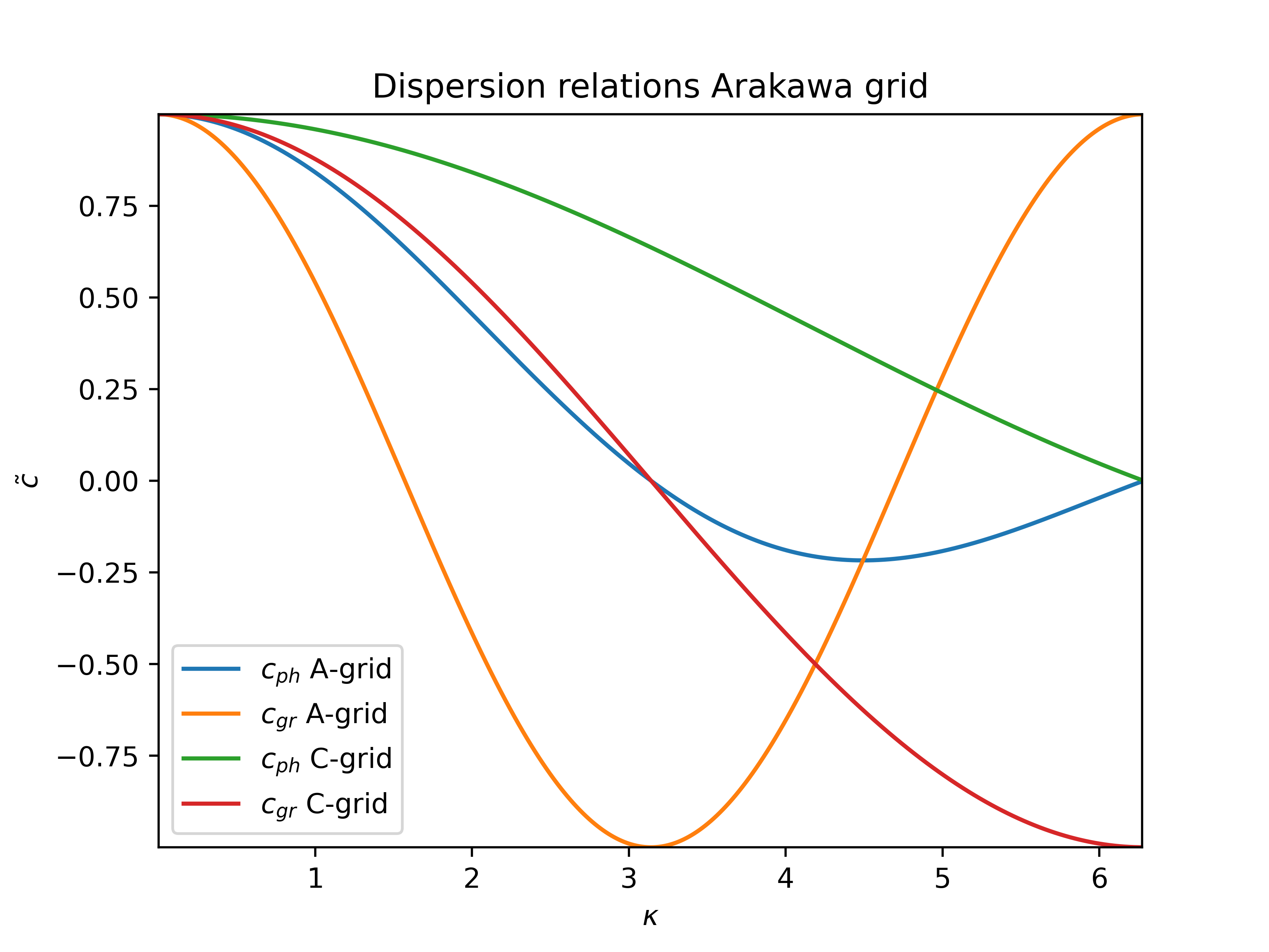
\[ \begin{align} \newtilde{c}_\text{ph} = \sqrt{2\frac{1 - \cos\left(\kappa\right)}{\left(\kappa\right)^2}}, & {} & \newtilde{c}_\text{gr} = \frac{\sin\left(\kappa\right)}{\sqrt{2 - 2\cos\left(\kappa\right)}} \end{align} \]
Fig. 26.2 shows the dispersion relations of the A-grid and the C-grid.
26.5 Scalar conservation properties on the C-grid
If $q$ is a conserved quantity, i.e. a quantity for which $\md{q} = 0$, then one can derive a continuity equation for $\newtilde{q} \coloneqq \rho q$:
\[ \begin{align} \md{q} = \frac{\partial q}{\partial t} + \mathbf{v}\cdot\nabla q &= 0,\\ \frac{\partial\rho}{\partial t} + \mathbf{v}\cdot\nabla \rho + \rho\nabla\cdot\mathbf{v} &= 0,\\ \Rightarrow \frac{\partial\newtilde{q}}{\partial t} + \nabla\cdot \mathbf{j}_{\newtilde{q}} &= 0, \end{align} \]
where the quantity $\mathbf{j}_{\newtilde{q}} \coloneqq \newtilde{q}\mathbf{v}$ denotes the flux of the quantity $q$. Defining
\[ \begin{align} Q \coloneqq \int_A\newtilde{q}d^3r \end{align} \]
as the global integral of the quantity $q$, $Q$ is conserved under kinematic boundary conditions:
\[ \begin{align} \frac{dQ}{dt} = -\int_A\nabla\cdot \mathbf{j}_{\newtilde{q}}d^3r = -\int_{\partial A}\mathbf{j}_{\newtilde{q}}\cdot d\mathbf{n} \end{align} \]
If one now decomposes $A$ into $N \geq 1$ grid boxes $A = A_1 \cup A_2 \cup \dots \cup A_N$, then the following holds
\[ \begin{align} Q = \sum_{i = 1}^NQ_i \end{align} \]
with
\[ \begin{align} Q_i\coloneqq\int_{A_i}\newtilde{q}d^3r. \end{align} \]
Thus one has
\[ \begin{align} \frac{dQ}{dt} = \sum_{i = 1}^N\frac{dQ_i}{dt} = -\sum_{i = 1}^N\int_{\partial A_i}\mathbf{j}_{\newtilde{q}}\cdot d\mathbf{n} = -\sum_{i = 1}^N\sum_{F \in F_i}\mathbf{j}_{\newtilde{q}}\cdot\mathbf{n}_F, \end{align} \]
where $F_i$ is the set of all side surfaces of the grid box $i$, and $\mathbf{n}_F$ is the normal vector perpendicular to the surface $F$ (pointing outwards). It is assumed that each $\partial A_i$ consists of a number of smooth surfaces over which one must sum individually, since they are separated by edges. Since each surface $F$ occurs twice in the double sum, but the vector $\mathbf{n}$ then points in two opposite directions, the sum amounts to zero, so that on a C-grid, even after discretization,
\[ \begin{align} Q = \text{const.} \end{align} \]
holds. Surfaces that are part of $\partial A$ trivially pose no problem, because by definition no mass flux occurs through them at all under kinematic boundary conditions. This is still true even under the generalized assumption that $\mathbf{j}_{\newtilde{q}}$ consists not only of $\newtilde{q}\mathbf{v}$, but of further, in particular diffusive, fluxes. It should also be noted that $Q$ remains a conserved quantity even if grid geometries are computed incorrectly.
26.6 Gradient fields on the C-grid
Let $\psi$ be a scalar field and $\nabla\psi$ the gradient of this scalar field, which is a vector field. On the C-grid, the rotation of a vector field $\mathbf{v}$ is determined by applying Stokes' theorem to a polygon with area $A$ and edge lengths $l_i$. Thus one has
\[ \begin{align} \mathbf{k}\cdot\nabla\times\mathbf{v} = \frac{1}{A}\sum_{i}\gamma_il_iv_i, \end{align} \]
where $v_i$ is the value of $\mathbf{v}$ at edge $i$ and $\gamma_i = 1$ if the unit vector of the edge points in the mathematically positive direction of circulation around the polygon, otherwise $\gamma_i = -1$. For the sake of simplicity, one assumes without loss of generality that $\gamma_i = 1$ for all $i$, so that one can write
\[ \begin{align} \mathbf{k}\cdot\nabla\times\mathbf{v} = \frac{1}{A}\sum_{i}l_iv_i \end{align} \]
Now one makes the ansatz
\[ \begin{align} \mathbf{v} = \nabla\psi \end{align} \]
which leads to
\[ \begin{align} \mathbf{k}\cdot\nabla\times\mathbf{v} = \frac{1}{A}\sum_{i}l_i\left(\nabla\psi\right)_i\tag{26.48}\label{eq:c-grid_rot_kons_deriv_0} \end{align} \]
One has
\[ \begin{align} \left(\nabla\psi\right)_i = \frac{\psi_{\text{to}\left(i\right)} - \psi_{\text{from}\left(i\right)}}{l_i}. \end{align} \]
Inserting this into Eq. (26.48), one obtains
\[ \begin{align} \mathbf{k}\cdot\nabla\times\psi = \frac{1}{A}\sum_{i}l_i\frac{\psi_{\text{to}\left(i\right)} - \psi_{\text{from}\left(i\right)}}{l_i} = \frac{1}{A}\sum_{i}\psi_{\text{to}\left(i\right)} - \psi_{\text{from}\left(i\right)}.\tag{26.50}\label{eq:c-grid_rot_kons_deriv_1} \end{align} \]
If one sorts the edges in the mathematically positive direction of circulation around the polygon under consideration, then the following holds
\[ \begin{align} \psi_{\text{to}\left(i\right)} = \psi_{\text{from}\left(i + 1\right)}. \end{align} \]
Every value of $\psi$ thus occurs twice in Eq. (26.50), once with a positive sign and once with a negative sign. This holds regardless of the spatial direction considered. Thus, on a C-grid, the following holds:
\[ \begin{align} \nabla\times\nabla\psi = \mathbf{0}. \end{align} \]
26.7 Scalar product on the C-grid
First of all, this section assumes a rectangular C-grid. While the discretizations of gradient and divergence are unique on such a grid, this is not the case for the scalar product. As a requirement on the discretization of the scalar product, one demands that the identity
\[ \begin{align} \nabla\cdot\left(\psi\mathbf{v}\right) = \mathbf{v}\cdot\nabla\psi + \psi\nabla\cdot\mathbf{v} \end{align} \]
should carry over to the discretization.
26.7.1 One-dimensional case
The notation is taken from Sect. 26.4.2 with the replacement $h \to \psi$. Averaging cells on edges is simply the arithmetic mean
\[ \begin{align} \newtilde{\psi}_{j} = \frac{\psi_{j - 1/2} + \psi_{j + 1/2}}{2}, \end{align} \]
since the edge $j$ is located in the middle between the two cells $j - 1/2$ and $j + 1/2$. One now computes
\[ \begin{align} \nabla\cdot\left(\psi u\right) &= \frac{\newtilde{\psi}_{j + 1}u_{j + 1} - \newtilde{\psi}_{j}u_{j}}{\Delta x} = \frac{\left(\psi_{j + 3/2} + \psi_{j + 1/2}\right)u_{j + 1} - \left(\psi_{j + 1/2} + \psi_{j - 1/2}\right)u_{j}}{2\Delta x}\nonumber\\ &= \frac{\psi_{j + 3/2}u_{j + 1} - \psi_{j - 1/2}u_{j} + \psi_{j + 1/2}\left(u_{j + 1} - u_{j}\right)}{2\Delta x}\nonumber\\ &= \frac{\psi_{j + 3/2}u_{j + 1} - \psi_{j - 1/2}u_{j} - \psi_{j + 1/2}\left(u_{j + 1} - u_{j}\right) + 2\psi_{j + 1/2}\left(u_{j + 1} - u_{j}\right)}{2\Delta x}\nonumber\\ &= \frac{\left(\psi_{j + 3/2} - \psi_{j + 1/2}\right)u_{j + 1} - \left(\psi_{j - 1/2} - \psi_{j + 1/2}\right)u_{j} + 2\psi_{j + 1/2}\left(u_{j + 1} - u_{j}\right)}{2\Delta x}\nonumber\\ &= \frac{1}{2}\left[\frac{\psi_{j + 3/2} - \psi_{j + 1/2}}{\Delta x}u_{j + 1} + \frac{\psi_{j + 1/2} - \psi_{j - 1/2}}{\Delta x}u_{j}\right]+ \psi_{j + 1/2}\frac{u_{j + 1} - u_{j}}{\Delta x}\nonumber\\ &\stackrel{!}{=} \psi\nabla\cdot\left(u\right) + u\frac{\partial\psi}{\partial x}. \end{align} \]
The product rule thus carries over if one defines the scalar product $uv$ of two vector fields $u$, $v$ by
\[ \begin{align} \left(uv\right)_{j + 1/2} = \frac{u_jv_j + u_{j + 1}v_{j + 1}}{2} \end{align} \]
26.7.2 Three-dimensional rectangular case
Summing the derivation of the previous section over all three spatial directions, one obtains the analogous statement for the three-dimensional case, with a scalar product
\[ \begin{align} \mathbf{u}\cdot\mathbf{v} = \sum_{e\in c}\frac{u_ev_e}{2}, \end{align} \]
where $c$ is the set of all side surfaces $e$ of the box under consideration.
26.7.3 Two-dimensional orthogonal grid
Let $A_c$ be the area of the cell $c$, $e$ an edge of the cell, $o\left(e\right)$ the neighboring cell of $c$ bordering the edge $e$, $d_e$ a dual edge length, and $l_e$ a primary edge length. One first writes
\[ \begin{align} \nabla\cdot\left(\psi\mathbf{v}\right) &= \frac{1}{A_c}\sum_{e\in c}l_e\frac{\psi_{o(e)} + \psi_c}{2}u_e,\\ \psi\nabla\cdot\mathbf{v} &= \frac{\psi_c}{A_c}\sum_{e\in c}l_eu_e. \end{align} \]
One now requires
\[ \begin{align} \mathbf{v}\cdot\nabla\psi &\stackrel{!}{=} \nabla\cdot\left(\psi\mathbf{v}\right) - \psi\nabla\cdot\mathbf{v}\nonumber\\ \Leftrightarrow\mathbf{v}\cdot\nabla\psi &= \frac{1}{A_c}\sum_{e\in c}l_e\frac{\psi_{o(e)} + \psi_c}{2}u_e - \frac{\psi_c}{A_c}\sum_{e\in c}l_eu_e = \frac{1}{A_c}\sum_{e\in c}l_e\frac{\psi_{o(e)} - \psi_c}{2}u_e = \frac{1}{A_c}\sum_{e\in c}\frac{\psi_{o(e)} - \psi_c}{d_e}u_e\frac{l_ed_e}{2}\nonumber\\ &= \sum_{e\in c}\frac{l_ed_e}{2A_c}\frac{\psi_{o(e)} - \psi_c}{d_e}u_e. \end{align} \]
From this one derives
\[ \begin{align} \left(\mathbf{u}\cdot\mathbf{v}\right)_c = \sum_{e\in c}\frac{l_ed_e}{2A_c}u_ev_e \end{align} \]
as the discretization for the scalar product. In the planar case, the sum of the weighting factors is
\[ \begin{align} \sum_{e\in c}\frac{l_ed_e}{2A_c} = 2. \end{align} \]
In a curved case, such as for example a spherical surface, this is however in general no longer the case.
26.7.4 Three-dimensional orthogonal grid (shallow)
Now the derivation in the previous section is generalized to a three-dimensional grid whose layer thickness $\Delta z_k$ depends only on the vertical index $k$. Vertical vector components are denoted by $w$, the index $u$ denotes the vector or scalar grid point above the grid box under consideration, the index $l$ denotes the respective grid point below. This leads to
\[ \begin{align} \nabla\cdot\left(\psi\mathbf{v}\right) &= \frac{1}{A_c\Delta z_k}\left(\sum_{e\in c}l_e\Delta z_k\frac{\psi_{o(e)} + \psi_c}{2}u_e + A_c\frac{\psi_u + \psi_c}{2}w_u - A_c\frac{\psi_l + \psi_c}{2}w_l\right),\tag{26.63}\label{eq:div_c-grid_shallow_no_terrain}\\ \psi\nabla\cdot\mathbf{v} &= \frac{\psi_c}{A_c\Delta z_k}\left(\sum_{e\in c}l_e\Delta z_ku_e + A_cw_u - A_cw_l\right). \end{align} \]
One again requires
\[ \begin{align} \mathbf{v}\cdot\nabla\psi &\stackrel{!}{=} \nabla\cdot\left(\psi\mathbf{v}\right) - \psi\nabla\cdot\mathbf{v}\nonumber\\ \Leftrightarrow\mathbf{v}\cdot\nabla\psi &= \frac{1}{A_c\Delta z_k}\left(\sum_{e\in c}l_e\Delta z_k\frac{\psi_{o(e)} + \psi_c}{2}u_e + A_c\frac{\psi_u + \psi_c}{2}w_u - A_c\frac{\psi_l + \psi_c}{2}w_l - \psi_c\sum_{e\in c}l_e\Delta z_ku_e - \psi_cA_cw_u + \psi_cA_cw_l\right)\nonumber\\ \Leftrightarrow\mathbf{v}\cdot\nabla\psi &= \frac{1}{A_c\Delta z_k}\left(\sum_{e\in c}l_e\Delta z_k\frac{\psi_{o(e)} - \psi_c}{2}u_e + A_c\frac{\psi_u - \psi_c}{2}w_u + A_c\frac{\psi_c - \psi_l}{2}w_l\right)\nonumber\\ \Leftrightarrow\mathbf{v}\cdot\nabla\psi &= \sum_{e\in c}\frac{l_ed_e}{2A_c}\frac{\psi_{o(e)} - \psi_c}{d_e}u_e + \frac{\Delta z_{k - 1/2}}{2\Delta z_k}\frac{\psi_u - \psi_c}{\Delta z_{k - 1/2}}w_u + \frac{\Delta z_{k + 1/2}}{2\Delta z_k}\frac{\psi_c - \psi_l}{\Delta z_{k + 1/2}}w_u. \end{align} \]
From this one derives
as the discretization for the scalar product in the shallow atmosphere. In the planar case, the sum of the weighting factors is
\[ \begin{align} \sum_{e\in c}\frac{l_ed_e}{2A_c} + \frac{\Delta z_{k - 1/2} + \Delta z_{k + 1/2}}{2\Delta z_k} = 3, \end{align} \]
where
\[ \begin{align} \Delta z_k &= z_{k - 1/2} - z_{k + 1/2} = \frac{z_{k - 1} + z_k}{2} - \frac{z_{k} + z_{k + 1}}{2} = \frac{z_{k - 1} + z_k - z_{k} - z_{k + 1}}{2}\nonumber\\ &= \frac{z_{k - 1} - z_{k} + z_k - z_{k + 1}}{2} = \frac{\Delta z_{k - 1/2} + \Delta z_{k + 1/2}}{2} \end{align} \]
was used. In a curved case, such as for example a spherical surface, this is however in general no longer the case.
26.7.5 Three-dimensional orthogonal grid (deep)
Now the derivation of the previous section is generalized to the deep atmosphere, i.e. the shallow atmosphere approximation is dropped. It is again assumed that the layer thickness $\Delta z_k$ only depends on the vertical index $k$. Using the same index notation as in the previous section one obtains
\[ \begin{align} \nabla\cdot\left(\psi\mathbf{v}\right) &= \frac{1}{V_{c, k}}\left(\sum_{e\in c}A_{e, k}\frac{\psi_{o(e)} + \psi_c}{2}u_{e, k} + A_{c, k + 1/2}\frac{\psi_{c, k} + \psi_{c, k - 1}}{2}w_{c, k + 1/2} - A_{c, k + 1/2}\frac{\psi_{c, k - 1} + \psi_{c, k}}{2}w_{c, k + 1/2}\right),\tag{26.69}\label{eq:div_c-grid_deep_no_terrain}\\ \psi\nabla\cdot\mathbf{v} &= \frac{\psi_c}{V_{c, k}}\left(\sum_{e\in c}A_{e, k}u_{e, k} + A_{c, k + 1/2}w_{c, k + 1/2} - A_{c, k + 1/2}w_{c, k + 1/2}\right). \end{align} \]
The cell base area $A_{c, k + 1/2}$ now also depends on the vertical index. $A_{e, k}$ is the vertical surface whose subset is the edge $\left(e, k\right)$. One again requires
\[ \begin{align} \mathbf{v}\cdot\nabla\psi &\stackrel{!}{=} \nabla\cdot\left(\psi\mathbf{v}\right) - \psi\nabla\cdot\mathbf{v}\nonumber\\ \Leftrightarrow\mathbf{v}\cdot\nabla\psi &= \frac{1}{V_{c, k}}\Bigg(\sum_{e\in c}A_{e, k}\frac{\psi_{o(e), k} + \psi_{c, k}}{2}u_{e, k} + A_{c, k + 1/2}\frac{\psi_{c, k} + \psi_{c, k - 1}}{2}w_{c, k + 1/2} - A_{c, k + 1/2}\frac{\psi_{c, k - 1} + \psi_{c, k}}{2}w_{c, k + 1/2}\nonumber\\ &- \sum_{e\in c}A_{e, k}\psi_{c, k}u_{e, k} - A_{c, k + 1/2}\psi_{c, k}w_{c, k + 1/2} + A_{c, k + 1/2}\psi_{c, k}w_{c, k + 1/2}\Bigg)\nonumber\\ \Leftrightarrow\mathbf{v}\cdot\nabla\psi &= \frac{1}{V_{c, k}}\left(\sum_{e\in c}A_{e, k}\frac{\psi_{o(e), k} - \psi_{c, k}}{2}u_{e, k} + A_{c, k + 1/2}\frac{\psi_{c, k - 1} - \psi_{c, k}}{2}w_{c, k + 1/2} + A_{c, k + 1/2}\frac{\psi_{c, k} - \psi_{c, k + 1}}{2}w_{c, k + 1/2}\right)\nonumber\\ \Leftrightarrow\mathbf{v}\cdot\nabla\psi &= \sum_{e\in c}\frac{A_{e, k}d_{e, k}}{2V_{c, k}}\frac{\psi_{o(e), k} - \psi_{c, k}}{d_{e, k}}u_{e, k} + \frac{A_{c, k + 1/2}\Delta z_{k - 1/2}}{2V_{c, k}}\frac{\psi_{c, k - 1} - \psi_{c, k}}{\Delta z_{k - 1/2}}w_{c, k + 1/2}\nonumber\\ &+ \frac{A_{c, k + 1/2}\Delta z_{k + 1/2}}{2V_{c, k}}\frac{\psi_{c, k} - \psi_{c, k + 1}}{\Delta z_{k + 1/2}}w_{c, k + 1/2}. \end{align} \]
From this one derives
\[ \begin{align} \mathbf{u}^{(1)}\cdot\mathbf{u}^{(2)} &= \sum_{e\in c}\frac{A_{e, k}d_{e, k}}{2V_{c, k}}u_{e, k}^{(1)}u_{e, k}^{(2)} + \frac{A_{c, k + 1/2}\Delta z_{k - 1/2}}{2V_{c, k}}w_{c, k + 1/2}^{(1)}w_{c, k + 1/2}^{(2)}\nonumber\\ &+ \frac{A_{c, k + 1/2}\Delta z_{k + 1/2}}{2V_{c, k}}w_{c, k + 1/2}^{(1)}w_{c, k + 1/2}^{(2)}\tag{26.72}\label{eq:inner_c-grid_3d_deep} \end{align} \]
as the discretization for the scalar product.
26.8 Choosing the C-grid
In summary, the C-grid has three advantages over the other grids:
It has advantageous dispersion relations.
Conservation of scalar variables is easy to ensure.
Gradient fields are irrotational.
The product rule $\nabla\cdot\left(\psi\mathbf{v}\right) = \mathbf{v}\cdot\nabla\psi + \psi\nabla\cdot\mathbf{v}$ reproduces itself under a suitable discretization of the scalar product.
Therefore, the decision is made at this point to use a C-grid for the dynamic core to be developed in part VII.
26.8.1 Conclusions
In a C-grid, the vectors are located on the edges and intersect them orthogonally. Extending the vector arrows in both directions, one ends up at the scalar data points. The grid obtained in this way is the so-called dual grid. Grids that possess a dual grid are called orthogonal. This is not always the case. In order to be able to exploit the favorable properties of the C-grid, one commits at this point to an orthogonal grid for the dynamic core to be formulated in part VII.
26.9 The problem of the ratio of degrees of freedom
In the continuous case, for $N \geq 1$ prognostic variables $\psi_i$ with $1 \leq i \leq N$ there is a system of $N$ prognostic equations. Linearizing these, a linear coupled system of partial differential equations arises. If no external forcings are included, it is homogeneous. If one inserts a plane wave $\psi_i = \newhat{\psi}_i\exp\left(i\mathbf{k}\cdot\mathbf{r} - i\omega t\right)$ with $\newhat{\psi}_i\in\mathbb{C}$ for each of the prognostic variables, a homogeneous linear system of equations for the complex amplitudes $\newhat{\psi}_i$ arises. This is an eigenvalue problem for the frequency $\omega$. The eigenvalues can be found by setting the characteristic polynomial (the determinant) of this system of equations to zero. According to the fundamental theorem of algebra, the characteristic polynomial has $N$ complex, though not necessarily distinct, zeros. Each of the distinct zeros corresponds to a branch of the dispersion relation.
When discretizing, this is particularly important when staggering vector fields. In the case of the linearized shallow water equations, one has three equations for the three variables $\left(u, v, h\right)$, so one has „twice as many arrows as points“. If a grid has too few arrows, the dispersion relation can no longer contain the necessary number of modes. If there are too many arrows, the dispersion relation could contain additional, unphysical branches. However, this can be prevented by applying special averaging operators in the prognostic equations.
26.9.1 Conclusions
On the triangular grid, one has 1.5 vector points per scalar grid point, whereas the correct ratio is 2. Such grids are therefore excluded. Quadrilateral grids are optimal in this respect. For grids with more than four vertices, one has to eliminate the overspecification by $m$ algebraic conditions on vector fields (one could also say: diagnostic equations or equations of state) per scalar grid point. For $N$ vertices, one has
\[ \begin{align} m = \frac{N - 4}{2}, \end{align} \]
since two cells each share an edge. For odd $N$, $m$ lies midway between two natural numbers, so that in this case a diagnostic vector equation would have to hold for two cells, which destroys the isotropy of the grid. It is therefore necessary that $N$ be even. Furthermore, one wants, if possible, to impose only one additional algebraic condition on vector fields per cell, so the first choice for $N$ is 4 and the second choice is 6.
The problem discussed in this section will be formulated in more detail in the next chapter for the hexagonal grid.
26.10 Exclusion of quadrilateral grids
The simplest quadrilateral grid is the longitude-latitude grid already excluded in Sect. 26.1. One finds that all known quadrilateral grids have at least one of the following fundamental problems, which have already been identified as exclusion criteria:
Orthogonality is violated (e.g. with the cubed-sphere grid)
Quasi-uniformity is violated (e.g. with the longitude-latitude grid).
Isotropy is grossly violated (e.g. with the kite grid).
The grid has edges or points where the structure deviates greatly from the grid structure in other regions (e.g. in the reduced longitude-latitude grid).
Therefore, quadrilateral grids are excluded at this point.
26.11 Choosing the hexagonal icosahedral grid
The only grid remaining after this elimination process is the hexagonal icosahedral grid.