23 Cloud microphysics

The so-called cloud microphysics is about answering the following questions:

• How do clouds and precipitation form?
• What size spectra do clouds and precipitation have?
• What is the falling speed of clouds and precipitation?
• What interactions exist between the condensates?

23.1 Köhler equation

The vapor pressure over a solution is given by equation (5.268):

\[ \begin{align} \ln\left(\frac{p_S\left(n_s\right)}{p_S^{(0)}}\right) &= -\frac{n_s}{n_w}. \end{align} \]

The notation was adapted to that common in cloud physics.

The vapor pressure over a curved surface is given by equation (5.301):

\[ \begin{align} \ln\left(\frac{p_S\left(R\right)}{p_S^{(0)}}\right) &= \frac{2\gamma}{R_sTR\rho_w}. \end{align} \]

If both effects occur at the same time, you get

\[ \begin{align} \ln\left(\frac{p_S\left(R,n_s\right)}{p_S^{(0)}}\right) &= \frac{2\gamma}{R_sTR\rho_w} - \frac{n_s}{n_w} \end{align} \]

as an equation for the vapor pressure over a curved surface within which a solution is located. For $n_w$ holds

\[ \begin{align} n_w = \frac{m_w}{M_w} = \frac{4\pi R^3\rho_w}{3M_w}. \end{align} \]

From this it follows

\[ \begin{align} \ln\left(\frac{p_S\left(R,n_s\right)}{p_S^{(0)}}\right) &= \frac{2\gamma}{R_sTR\rho_w} - \frac{3M_wn_s}{4\pi R^3\rho_w}. \end{align} \]

If you use the diameter $D$ instead of the radius $R$, it follows

This equation is called Köhler equation.

If you derive this equation in terms of $D$ and set the derivative equal to zero, you get

\[ \begin{align} 0 &= -\frac{4\gamma}{R_sTD_c^2\rho_w} + \frac{18M_wn_s}{\pi D_c^4\rho_w}\nonumber\\ \Leftrightarrow \frac{4\gamma}{R_sTD_c^2} &= \frac{18M_wn_s}{\pi D_c^4}\nonumber\\ \Leftrightarrow \frac{4\gamma D_c^2}{R_sT} &= \frac{18M_wn_s}{\pi}\nonumber\\ \Leftrightarrow D_c^2 &= \frac{9R_sTM_wn_s}{2\gamma\pi} = \frac{9RTn_s}{2\gamma\pi}. \end{align} \]

$D_c$ is called critical diameter. The saturation vapor pressure is maximum at the critical diameter. Only drops with $D>D_c$ can continue to grow and become cloud and rain drops. Such drops only form in the free atmosphere for $p_v>p_S\left(D_c\right)$.

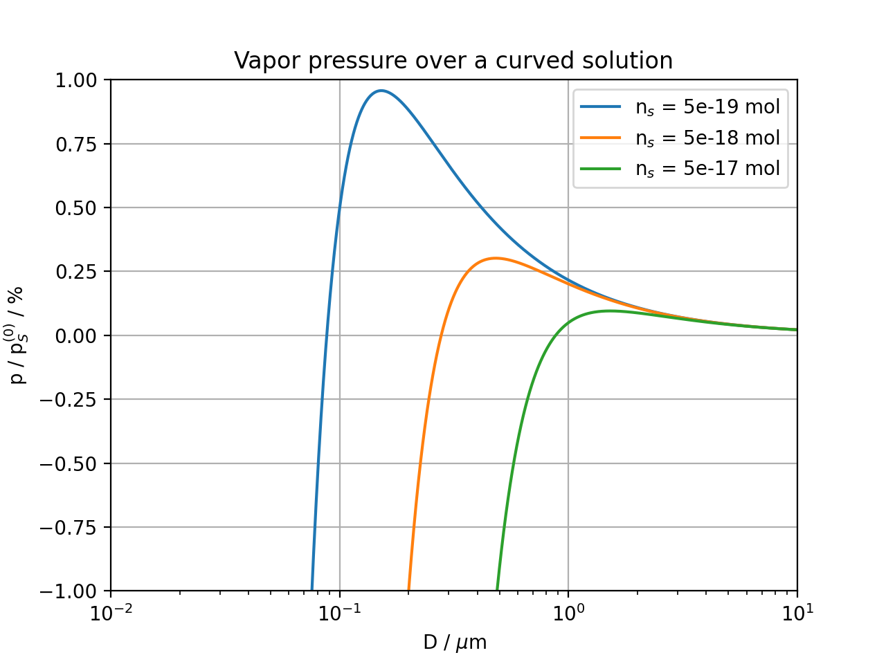
As can be seen from Fig. 23.1, the critical diameter increases with $n_s$, whereas the maximum saturation vapor pressure decreases.

23.2 Circulation around condensates

From the flow field around a condensate you can derive the force that acts on the condensate, which results in the falling speed by equating it with the weight.

23.2.1 Laminar flow

Imagine a sphere with radius $a$ centered at the origin of a Cartesian coordinate system. One now looks for solutions to the imcompressible system of equations without momentum advection

with the boundary conditions

One limits oneself to stationary, i.e. especially laminar solutions. This results in the momentum equation Eq. (23.8)

\[ \begin{align} \nabla p &= \eta\Delta\mathbf{v}.\tag{23.12}\label{eq:momentum_for_stokes_mod} \end{align} \]

The notation of $\mathbf{v}$ in spherical coordinates is

\[ \begin{align} \mathbf{v} &= v_r\mathbf{e}_r + v_\theta\mathbf{e}_\theta + v_\phi\mathbf{e}_\phi. \end{align} \]

Here $\theta$ is the angle relative to the z-axis and $\phi$ is the angle relative to the xz-plane. Stationary solutions are rotationally symmetrical about the z-axis, and the following also applies

\[ \begin{align} v_\phi = 0. \end{align} \]

The following applies to the friction force created by the flow, which acts on the ball

\[ \begin{align} F = -2\pi a^2\int_0^\pi\left[p\cos\left(\theta\right) + \eta\sin\left(\theta\right)\frac{\partial v_\theta}{\partial r}\right]\sin\left(\theta\right)d\theta. \end{align} \]

Such a friction force is called Stokes friction. This is divided into a force $F_p$, which arises from the pressure $p$, and a force $F_v$, which arises from the shear of the velocity field, i.e

\[ \begin{align} F_p &\coloneqq -2\pi a^2\int_0^\pi p\cos\left(\theta\right)\sin\left(\theta\right)d\theta,\tag{23.16}\label{eq:stokes_friction_p}\\ F_v &\coloneqq -2\pi\eta a^2\int_0^\pi\frac{\partial v_\theta}{\partial r}\sin\left(\theta\right)^2d\theta.\tag{23.17}\label{eq:stokes_friction_v} \end{align} \]

This applies

\[ \begin{align} F = F_p + F_v.\tag{23.18}\label{eq:stokes_friction_split-up} \end{align} \]

According to the statements at the beginning of Chap. 15 and Eq. (23.9) can be $\mathbf{v}$ in the form

\[ \begin{align} \mathbf{v} = \nabla\times\mathbf{A} \end{align} \]

represented by a velocity potential $\mathbf{A}$. According to Eq. (B.98) applies

\[ \begin{align} \nabla\times\mathbf{A} &= \frac{A_\theta}{r}\mathbf{e}_\phi + \frac{A_\phi}{r\tan\left(\theta\right)}\mathbf{e}_r - \frac{A_\phi}{r}\mathbf{e}_\theta + \mathbf{e}_r\left(\frac{1}{r}\frac{\partial A_\phi}{\partial\theta} - \frac{1}{r\sin\left(\theta\right)}\frac{\partial A_\theta}{\partial\phi}\right)\nonumber\\ & + \mathbf{e}_\theta\left(\frac{1}{r\sin\left(\theta\right)}\frac{\partial A_r}{\partial\phi} - \frac{\partial A_\phi}{\partial r}\right) + \mathbf{e}_\phi\left(\frac{\partial A_\theta}{\partial r} - \frac{1}{r}\frac{\partial A_r}{\partial\theta}\right). \end{align} \]

Due to rotational symmetry about the z-axis, $\mathbf{v}$ does not depend on $\phi$. This implies

\[ \begin{align} \nabla\times\mathbf{A} &= \frac{A_\theta}{r}\mathbf{e}_\phi + \frac{A_\phi}{r\tan\left(\theta\right)}\mathbf{e}_r - \frac{A_\phi}{r}\mathbf{e}_\theta + \mathbf{e}_r\frac{1}{r}\frac{\partial A_\phi}{\partial\theta} - \mathbf{e}_\theta\frac{\partial A_\phi}{\partial r} + \mathbf{e}_\phi\left(\frac{\partial A_\theta}{\partial r} - \frac{1}{r}\frac{\partial A_r}{\partial\theta}\right). \end{align} \]

By projections onto the location-dependent basis elements of the spherical coordinates one obtains

\[ \begin{align} v_r &= \frac{A_\phi}{r\tan\left(\theta\right)} + \frac{1}{r}\frac{\partial A_\phi}{\partial\theta},\\ v_\theta &= -\frac{A_\phi}{r} - \frac{\partial A_\phi}{\partial r},\\ v_\phi &= \frac{A_\theta}{r} + \frac{\partial A_\theta}{\partial r} - \frac{1}{r}\frac{\partial A_r}{\partial\theta}. \end{align} \]

The condition $v_\phi = 0$ can therefore be fulfilled by $A_\theta = A_r = 0$ without affecting the other components. Define

\[ \begin{align} \psi = \psi\left(r, \theta\right) \coloneqq -rA_\phi\sin\left(\theta\right), \end{align} \]

then applies

The rotation of the wind field is:

\[ \begin{align} \nabla\times\mathbf{v} &= \frac{v_\theta}{r}\mathbf{e}_\phi + \frac{v_\phi}{r\tan\left(\theta\right)}\mathbf{e}_r - \frac{v_\phi}{r}\mathbf{e}_\theta + \mathbf{e}_r\frac{1}{r}\frac{\partial v_\phi}{\partial\theta} - \mathbf{e}_\theta\frac{\partial v_\phi}{\partial r} + \mathbf{e}_\phi\left(\frac{\partial v_\theta}{\partial r} - \frac{1}{r}\frac{\partial v_r}{\partial\theta}\right). \end{align} \]

With $v_\phi = 0$ it follows from this

\[ \begin{align} \zetabi = \nabla\times\mathbf{v} &= \frac{v_\theta}{r}\mathbf{e}_\phi + \mathbf{e}_\phi\left(\frac{\partial v_\theta}{\partial r} - \frac{1}{r}\frac{\partial v_r}{\partial\theta}\right) = \mathbf{e}_\phi\left(\frac{\partial v_\theta}{\partial r} - \frac{1}{r}\frac{\partial v_r}{\partial\theta} + \frac{v_\theta}{r}\right). \end{align} \]

If you insert the equations (23.26) - (23.27) here, you get

\[ \begin{align} \zetabi &= \nabla\times\mathbf{v} = \mathbf{e}_\phi\left(\frac{1}{r\sin\left(\theta\right)}\frac{\partial^2\psi}{\partial r^2} - \frac{1}{r^2\sin\left(\theta\right)}\frac{\partial\psi}{\partial r} - \frac{\cos\left(\theta\right)}{r^3\sin\left(\theta\right)^2}\frac{\partial\psi}{\partial\theta} + \frac{1}{r^3\sin\left(\theta\right)}\frac{\partial^2\psi}{\partial\theta^2} + \frac{1}{r^2\sin\left(\theta\right)}\frac{\partial\psi}{\partial r}\right)\nonumber\\ &= \mathbf{e}_\phi\left(\frac{1}{r\sin\left(\theta\right)}\frac{\partial^2\psi}{\partial r^2} - \frac{\cos\left(\theta\right)}{r^3\sin\left(\theta\right)^2}\frac{\partial\psi}{\partial\theta} + \frac{1}{r^3\sin\left(\theta\right)}\frac{\partial^2\psi}{\partial\theta^2}\right)\nonumber\\ &= \frac{\mathbf{e}_\phi}{r\sin\left(\theta\right)}\left(\frac{\partial^2\psi}{\partial r^2} - \frac{\cos\left(\theta\right)}{r^2\sin\left(\theta\right)}\frac{\partial\psi}{\partial\theta} + \frac{1}{r^2}\frac{\partial^2\psi}{\partial\theta^2}\right)\nonumber\\ &= \frac{\mathbf{e}_\phi}{r\sin\left(\theta\right)}\left[\frac{\partial^2}{\partial r^2} + \frac{\sin\left(\theta\right)}{r^2}\frac{\partial}{\partial\theta}\left(\frac{1}{\sin\left(\theta\right)}\frac{\partial}{\partial\theta}\right)\right]\psi \equiv \frac{\mathbf{e}_\phi}{r\sin\left(\theta\right)}E^2\psi \end{align} \]

with a differential operator

\[ \begin{align} E^2 \coloneqq \frac{\partial^2}{\partial r^2} - \frac{1}{r^2\tan\left(\theta\right)}\frac{\partial}{\partial\theta} + \frac{1}{r^2}\frac{\partial^2}{\partial\theta^2} = \frac{\partial^2}{\partial r^2} + \frac{\sin\left(\theta\right)}{r^2}\frac{\partial}{\partial\theta}\left(\frac{1}{\sin\left(\theta\right)}\frac{\partial}{\partial\theta}\right). \end{align} \]

From this it follows that:

\[ \begin{align} \zetabi &= \nabla\times\left(\nabla\times\mathbf{A}\right) = \nabla\times\left[\nabla\times\left(A_\phi\mathbf{e}_\phi\right)\right] = -\nabla\times\left[\nabla\times\left(\frac{\psi}{r\sin\left(\theta\right)}\mathbf{e}_\phi\right)\right]. \end{align} \]

For doubly continuously differentiable scalar fields $\chi$ therefore holds

\[ \begin{align} -\nabla\times\left[\nabla\times\left(\frac{\chi}{r\sin\left(\theta\right)}\mathbf{e}_\phi\right)\right] &= \frac{\mathbf{e}_\phi}{r\sin\left(\theta\right)}E^2\chi. \end{align} \]

Eq. (B.54) is

\[ \begin{align} \Delta\mathbf{v} &= \nabla\left(\nabla\cdot\mathbf{v}\right) - \nabla\times\left(\nabla\times\mathbf{v}\right) \stackrel{\href{#eq:incompressibility_stokes_fric}{\text{Glg. (23.9)}}}{=} -\nabla\times\left(\nabla\times\mathbf{v}\right) = -\nabla\times\zetabi. \end{align} \]

This allows the momentum equation Eq. (23.12) in the form

note down. If you apply the rotation again, it follows

\[ \begin{align} 0 = -\eta\nabla\times\left(\nabla\times\zetabi\right) = -\eta\nabla\times\left[\nabla\times\left(\frac{\mathbf{e}_\phi}{r\sin\left(\theta\right)}E^2\psi\right)\right] = \eta\frac{\mathbf{e}_\phi}{r\sin\left(\theta\right)}E^4\psi. \end{align} \]

So you can

use as the differential equation for $\psi$. From the boundary condition Eq. (23.11) follow

\[ \begin{align} \frac{\partial\psi}{\partial r}\left(r = a\right) &= 0,\tag{23.38}\label{eq:stokes_psi_bc_4}\\ \frac{\partial\psi}{\partial\theta}\left(r = a\right) &= 0. \end{align} \]

So $\psi$ is constant along the surface of the sphere, o. B. d. A. can be used as a boundary condition

\[ \begin{align} \psi\left(r = a\right) = 0\tag{23.40}\label{eq:stokes_psi_bc_1} \end{align} \]

demand. The boundary condition Eq. (23.10) is in spherical coordinates

\[ \begin{align} \lim_{\left|\mathbf{r}\right|\to\infty}v_r &= U\cos\left(\theta\right),\tag{23.41}\label{eq:stokes_psi_bc_2}\\ \lim_{\left|\mathbf{r}\right|\to\infty}v_\theta &= -U\sin\left(\theta\right).\tag{23.42}\label{eq:stokes_psi_bc_3} \end{align} \]

The pressure is said to converge at infinity to a homogeneous background pressure $p_0$:

\[ \begin{align} \lim_{\left|\mathbf{r}\right| \to \infty}p &= p_0 \end{align} \]

It applies

\[ \begin{align} E^4\psi &= \left(\frac{\partial^2}{\partial r^2} - \frac{1}{r^2\tan\left(\theta\right)}\frac{\partial}{\partial\theta} + \frac{1}{r^2}\frac{\partial^2}{\partial\theta^2}\right)\left(\frac{\partial^2\psi}{\partial r^2} - \frac{1}{r^2\tan\left(\theta\right)}\frac{\partial\psi}{\partial\theta} + \frac{1}{r^2}\frac{\partial^2\psi}{\partial\theta^2}\right).\tag{23.44}\label{eq:stokes_e4} \end{align} \]

Now you do the approach for $\psi$

\[ \begin{align} \psi\left(r,\theta\right) = -\frac{U\sin\left(\theta\right)^2}{2}\left(Ar + Br^2 + \frac{C}{r}\right).\tag{23.45}\label{eq:stokes_ansatz} \end{align} \]

From Eq. (23.41) follows

\[ \begin{align} \lim_{\left|\mathbf{r}\right| \to \infty}v_r &= -\lim_{\left|\mathbf{r}\right|\to\infty}\frac{1}{r^2\sin\left(\theta\right)}\frac{\partial\psi}{\partial\theta} = \lim_{\left|\mathbf{r}\right|\to\infty}\frac{1}{r^2\sin\left(\theta\right)}\frac{\partial}{\partial\theta}\frac{U\sin\left(\theta\right)^2}{2}\left(Ar + Br^2 + \frac{C}{r}\right)\nonumber\\ &= \lim_{\left|\mathbf{r}\right|\to\infty}\frac{1}{r^2\sin\left(\theta\right)}U\sin\left(\theta\right)\cos\left(\theta\right)\left(Ar + Br^2 + \frac{C}{r}\right)\nonumber\\ &= \lim_{\left|\mathbf{r}\right|\to\infty}U\cos\left(\theta\right)\left(\frac{A}{r} + B + \frac{C}{r^3}\right)\nonumber\\ &= \lim_{\left|\mathbf{r}\right|\to\infty}BU\cos\left(\theta\right) = BU\cos\left(\theta\right). \end{align} \]

Comparison with Eq. (23.41) implied

\[ \begin{align} B = 1. \end{align} \]

From Eq. (23.42) follows

\[ \begin{align} \lim_{\left|\mathbf{r}\right|\to\infty}v_\theta &= \lim_{\left|\mathbf{r}\right|\to\infty}\frac{1}{r\sin\left(\theta\right)}\frac{\partial\psi}{\partial r} = -\lim_{\left|\mathbf{r}\right|\to\infty}\frac{1}{r\sin\left(\theta\right)}\frac{\partial}{\partial r}\frac{U\sin\left(\theta\right)^2}{2}\left(Ar + Br^2 + \frac{C}{r}\right)\nonumber\\ &= -\lim_{\left|\mathbf{r}\right|\to\infty}\frac{1}{r\sin\left(\theta\right)}\frac{U\sin\left(\theta\right)^2}{2}\left(A + 2Br - \frac{C}{r^2}\right)\nonumber\\ &= -\lim_{\left|\mathbf{r}\right|\to\infty}U\sin\left(\theta\right)\left(\frac{A}{2r} + B - \frac{C}{2r^3}\right)\nonumber\\ &= -\lim_{\left|\mathbf{r}\right|\to\infty}U\sin\left(\theta\right)B = -BU\sin\left(\theta\right). \end{align} \]

Comparison with Eq. (23.42) again implies $B = 1$, so

\[ \begin{align} \psi\left(r,\theta\right) = -\frac{U\sin\left(\theta\right)^2}{2}\left(Ar + r^2 + \frac{C}{r}\right). \end{align} \]

From Eq. (23.40) is further obtained

\[ \begin{align} \psi\left(a,\theta\right) &= -\frac{U\sin\left(\theta\right)^2}{2}\left(Aa + a^2 + \frac{C}{a}\right) \hastobe 0\\ \Leftrightarrow Aa + a^2 + \frac{C}{a} &= 0\\ \Leftrightarrow Aa^2 + a^3 + C &= 0\\ \Leftrightarrow C &= -Aa^2 - a^3, \end{align} \]

so

\[ \begin{align} \psi\left(r,\theta\right) = -\frac{U\sin\left(\theta\right)^2}{2}\left(Ar + r^2 - \frac{Aa^2 + a^3}{r}\right). \end{align} \]

From this it follows

\[ \begin{align} \frac{\psi\left(r,\theta\right)}{\partial r} = -\frac{U\sin\left(\theta\right)^2}{2}\left(A + 2r + \frac{Aa^2 + a^3}{r^2}\right). \end{align} \]

From Eq. (23.38) follows

\[ \begin{align} A + 2a + \frac{Aa^2 + a^3}{a^2} = A + 2a + A + a &= 2A + 3a \hastobe 0\nonumber\\ \Leftrightarrow A &= -\frac{3a}{2}. \end{align} \]

So the approach is:

\[ \begin{align} \psi\left(r,\theta\right) &= -\frac{U\sin\left(\theta\right)^2}{2}\left(-\frac{3a}{2}r + r^2 + \frac{3a^3}{2r} - \frac{a^3}{r}\right)\nonumber\\ &= -\frac{U\sin\left(\theta\right)^2}{2}\left(-\frac{3a}{2}r + r^2 + \frac{a^3}{2r}\right).\tag{23.57}\label{eq:stokes_ansatz_concrete} \end{align} \]

Now this is shown in Eq. (23.44) is used. Preparatory calculations are made

\[ \begin{align} \frac{\partial^2\psi}{\partial r^2} &= -\frac{U\sin\left(\theta\right)^2}{2}\left(2 + \frac{a^3}{r^3}\right),\\ -\frac{1}{r^2\tan\left(\theta\right)}\frac{\partial\psi}{\partial\theta} &= U\cos\left(\theta\right)^2\left(-\frac{3a}{2r} + 1 + \frac{a^3}{2r^3}\right),\\ \frac{1}{r^2}\frac{\partial^2\psi}{\partial\theta^2} &= -U\left(\cos\left(\theta\right)^2 - \sin\left(\theta\right)^2\right)\left(-\frac{3a}{2r} + 1 + \frac{a^3}{2r^3}\right). \end{align} \]

Adding these three terms together gives

\[ \begin{align} E^2\psi &= \frac{\partial^2\psi}{\partial r^2} - \frac{1}{r^2\tan\left(\theta\right)}\frac{\partial\psi}{\partial\theta} + \frac{1}{r^2}\frac{\partial^2\psi}{\partial\theta^2} = -\frac{U\sin\left(\theta\right)^2}{2}\left(2 + \frac{a^3}{r^3}\right) + U\sin\left(\theta\right)^2\left(-\frac{3a}{2r} + 1 + \frac{a^3}{2r^3}\right)\\ &= -\frac{U\sin\left(\theta\right)^2}{2}\left(2 + \frac{a^3}{r^3} + \frac{3a}{r} - 2 - \frac{a^3}{r^3}\right)\\ &= -\frac{3aU\sin\left(\theta\right)^2}{2r}.\tag{23.63}\label{eq:stokes_e2} \end{align} \]

From this it follows

\[ \begin{align} \frac{\partial^2E^2\psi}{\partial r^2} &= -\frac{6aU\sin\left(\theta\right)^2}{2r^3} = -\frac{3aU\sin\left(\theta\right)^2}{r^3},\\ -\frac{1}{r^2\tan\left(\theta\right)}\frac{\partial E^2\psi}{\partial\theta} &= \frac{3aU\cos\left(\theta\right)^2}{r^3},\\ \frac{1}{r^2}\frac{\partial^2 E^2\psi}{\partial\theta^2} &= -\frac{3aU\left(\cos\left(\theta\right)^2 - \sin\left(\theta\right)^2\right)}{r^3}. \end{align} \]

Adding these three equations together, it follows

\[ \begin{align} E^4\psi = 0. \end{align} \]

Eq. (23.37) actually solves Eq. (23.37).

Now it remains to be shown that Eq. (23.35) from the approach Eq. (23.37) is solved. You first calculate this

\[ \begin{align} \nabla\times\zetabi &= \nabla\times\left[\mathbf{e}_\phi\frac{E^2\psi}{r\sin\left(\theta\right)}\right] \stackrel{\href{ch-40-vector-analysis.html#eq:diff_op_rule_5}{\text{Glg. (B.51)}}}{=} -\mathbf{e}_\phi\times\nabla\frac{E^2\psi}{r\sin\left(\theta\right)} + \frac{E^2\psi}{r\sin\left(\theta\right)}\nabla\times\mathbf{e}_\phi. \end{align} \]

With

\[ \begin{align} \nabla\times\mathbf{e}_\phi &\stackrel{\href{ch-40-vector-analysis.html#eq:rot_sphere}{\text{Glg. (B.98)}}}{=} \frac{1}{r\tan\left(\theta\right)}\mathbf{e}_r - \frac{1}{r}\mathbf{e}_\theta \end{align} \]

follows

\[ \begin{align} \nabla\times\zetabi &= -\mathbf{e}_\phi\times\nabla\frac{E^2\psi}{r\sin\left(\theta\right)} + \frac{E^2\psi}{r\sin\left(\theta\right)}\left(\frac{1}{r\tan\left(\theta\right)}\mathbf{e}_r - \frac{1}{r}\mathbf{e}_\theta\right)\nonumber\\ &= -\mathbf{e}_\phi\times\nabla\frac{E^2\psi}{r\sin\left(\theta\right)} + \frac{\cos\left(\theta\right)E^2\psi}{r^2\sin\left(\theta\right)^2}\mathbf{e}_r - \frac{E^2\psi}{r^2\sin\left(\theta\right)}\mathbf{e}_\theta. \end{align} \]

If you put Eq. (23.63), you get

\[ \begin{align} \nabla\times\zetabi &= -\frac{3aU}{2}\left(-\mathbf{e}_\phi\times\nabla\frac{\sin\left(\theta\right)}{r^2} + \frac{\cos\left(\theta\right)}{r^3}\mathbf{e}_r - \frac{\sin\left(\theta\right)}{r^3}\mathbf{e}_\theta\right).\tag{23.71}\label{eq:stokes_deriv_1} \end{align} \]

With Eq. (B.88) follows

\[ \begin{align} \nabla\frac{\sin\left(\theta\right)}{r^2} &= -\frac{2\sin\left(\theta\right)}{r^3}\mathbf{e}_r + \frac{\cos\left(\theta\right)}{r^3}\mathbf{e}_\theta. \end{align} \]

Therefore applies

\[ \begin{align} -\mathbf{e}_\phi\times\nabla\frac{\sin\left(\theta\right)}{r^2} &= \frac{2\sin\left(\theta\right)}{r^3}\mathbf{e}_\theta + \frac{\cos\left(\theta\right)}{r^3}\mathbf{e}_r. \end{align} \]

Putting this into Eq. (23.71), you get

\[ \begin{align} \nabla\times\zetabi &= -\frac{3aU}{2}\left(\frac{2\sin\left(\theta\right)}{r^3}\mathbf{e}_\theta + \frac{\cos\left(\theta\right)}{r^3}\mathbf{e}_r + \frac{\cos\left(\theta\right)}{r^3}\mathbf{e}_r - \frac{\sin\left(\theta\right)}{r^3}\mathbf{e}_\theta\right)\nonumber\\ &= -\frac{3aU}{2}\left(\frac{\sin\left(\theta\right)}{r^3}\mathbf{e}_\theta + \frac{2\cos\left(\theta\right)}{r^3}\mathbf{e}_r\right). \end{align} \]

Putting this into Eq. (23.35), you get

\[ \begin{align} \nabla p = \frac{3aU}{2}\frac{\eta\sin\left(\theta\right)}{r^3}\mathbf{e}_\theta + \frac{3aU}{2}\frac{2\eta\cos\left(\theta\right)}{r^2}\mathbf{e}_r, \end{align} \]

so

\[ \begin{align} \frac{\partial p}{\partial r} &= \frac{3aU}{2}\frac{2\eta\cos\left(\theta\right)}{r^3},\nonumber\\ \frac{\partial p}{\partial\theta} &= \frac{3aU}{2}\frac{\eta\sin\left(\theta\right)}{r^2}. \end{align} \]

This is solved by

\[ \begin{align} p = p_0 - \frac{3aU}{2}\frac{\eta\cos\left(\theta\right)}{r^2}. \end{align} \]

This implies for the friction force created by the pressure according to Eq. (23.16)

\[ \begin{align} F_p &= -2\pi a^2\int_0^\pi-\frac{3\eta aU\cos\left(\theta\right)}{2a^2}\cos\left(\theta\right)\sin\left(\theta\right)d\theta = \pi\int_0^\pi 3\eta aU\cos\left(\theta\right)\cos\left(\theta\right)\sin\left(\theta\right)d\theta\nonumber\\ &= 3\eta aU\pi\int_0^\pi\cos^2\left(\theta\right)\sin\left(\theta\right)d\theta = -3\eta aU\pi\left[\frac{1}{3}\cos\left(\theta\right)^3\right]_0^\pi = 2\eta aU\pi. \end{align} \]

For $v_\theta$ one obtains using Eq. (23.27) and the approach Eq. (23.57)

\[ \begin{align} v_\theta &= \frac{1}{r\sin\left(\theta\right)}\frac{\partial\psi}{\partial r} = \frac{1}{r\sin\left(\theta\right)}\frac{\partial}{\partial r}\left[-\frac{U\sin\left(\theta\right)^2}{2}\left(-\frac{3a}{2}r + r^2 + \frac{a^3}{2r}\right)\right]\nonumber\\ &= \frac{1}{r}\frac{\partial}{\partial r}\left[\frac{U\sin\left(\theta\right)}{2}\left(\frac{3a}{2}r - r^2 - \frac{a^3}{2r}\right)\right] = \frac{1}{r}\frac{\partial}{\partial r}\left[\frac{Ua^2\sin\left(\theta\right)}{2}\left(\frac{3}{2a}r - \frac{r^2}{a^2} - \frac{a}{2r}\right)\right]\nonumber\\ &= \frac{1}{r}\left[\frac{Ua^2\sin\left(\theta\right)}{4}\left(-\frac{4r}{a^2} + \frac{3}{a} + \frac{a}{r^2}\right)\right] = \frac{Ua^2\sin\left(\theta\right)}{4}\left(-\frac{4}{a^2} + \frac{3}{ar} + \frac{a}{r^3}\right). \end{align} \]

From this it follows

\[ \begin{align} \frac{\partial v_\theta}{\partial r} &= -\frac{Ua^2\sin\left(\theta\right)}{4}\left(\frac{3}{ar^2} + \frac{3a}{r^4}\right). \end{align} \]

If you evaluate this at $r = a$, it follows

\[ \begin{align} \frac{\partial v_\theta}{\partial r}\left(r = a\right) &= -\frac{Ua^2\sin\left(\theta\right)}{4}\left(\frac{3}{a^3} + \frac{3}{a^3}\right) = -\frac{6U\sin\left(\theta\right)}{4a} = -\frac{3U\sin\left(\theta\right)}{2a}. \end{align} \]

Putting this into Eq. (23.17), you get

\[ \begin{align} F_v &= -2\pi\eta a^2\int_0^\pi-\frac{3U\sin\left(\theta\right)}{2a}\sin\left(\theta\right)^2d\theta = 3U\pi\eta a\int_0^\pi\sin\left(\theta\right)^3d\theta. \end{align} \]

You now integrate

\[ \begin{align} \int_0^\pi\sin\left(\theta\right)^3d\theta &= \left[-\cos\left(\theta\right)\sin\left(\theta\right)^2\right]_0^\pi + 2\int_0^\pi\cos\left(\theta\right)^2\sin\left(\theta\right)d\theta\nonumber\\ &= 2\int_0^\pi\cos\left(\theta\right)^2\sin\left(\theta\right)d\theta = \frac{2}{3}\left[-\cos\left(\theta\right)^3\right]_0^\pi = \frac{2}{3}\left[\cos\left(\theta\right)^3\right]_\pi^0 = \frac{4}{3}. \end{align} \]

This implies

\[ \begin{align} F_v &= 3U\pi\eta a\frac{4}{3} = 4U\pi\eta a. \end{align} \]

Therefore, according to Eq. (23.18) for the friction force

If you put this with the weight

\[ \begin{align} F_g = mg = \frac{4}{3}\pi a^3\left(\rho_l' - \rho_h'\right)g\tag{23.86}\label{eq:gravity_on_condensate} \end{align} \]

equal, you get

as a formula for the equilibrium falling speed $v_F$. In Eq. (23.86) the static buoyancy of the condensate is subtracted.

23.2.2 Turbulent flow around

In the case of turbulent flow, the circulation surrounding the condensate is time-dependent in an aperiodic manner. Here the friction force $F$ is proportional to the square of the speed $U$,

\[ \begin{align} F = \frac{1}{2}c_w\pi a^2\rho_h'U^2,\tag{23.88}\label{eq:turbulent_friction} \end{align} \]

where $c_w \geq 0$ is a constant dependent on the shape of the object flowed around, the so-called $c_w-$value. In English this quantity is called drag coefficient $c_d$. If you compare this with the weight force according to Eq. (23.86) is equal, you get

\[ \begin{align} \frac{1}{2}c_w\pi a^2\rho_h'v_F^2 &= \frac{4}{3}\pi a^3\rho_l'g \Leftrightarrow v_F^2 = \frac{8a\rho_l'g}{3\rho_h'c_w} \end{align} \]

as a formula for the equilibrium falling speed $v_F$.

23.2.3 Compound formula for falling speed

Small condensates flow around laminarly, larger ones flow turbulently. The parameter $\alpha\in\left[0, 1\right]$ describes the proportion of turbulence in the friction force $F$, i.e

\[ \begin{align} F = \alpha F_\text{turbulent} + \left(1 - \alpha\right)F_\text{laminar}. \end{align} \]

If you insert the equations (23.85) and (23.88) here, you get

\[ \begin{align} F = \alpha\frac{1}{2}c_w\pi a^2\rho_h'U^2 + \left(1 - \alpha\right)6\pi a\rho_h'\nu U. \end{align} \]

Here $c_w \approx 0.8$ is a realistic value. If you compare this with the weight force according to Eq. (23.86) is the same, assuming $\alpha \not= 0$

\[ \begin{align} \left(1 - \alpha\right)6\pi a\rho_h'\nu v_F + \alpha\frac{1}{2}c_w\pi a^2\rho_h'v_F^2 &= \frac{4}{3}\pi a^3\rho_l'g\nonumber\\ \Leftrightarrow\alpha\frac{1}{2}c_w\pi a\rho_h'v_F^2 + \left(1 - \alpha\right)6\pi\rho_h'\nu v_F - \frac{4}{3}\pi a^2\rho_l'g &= 0\nonumber\\ \Leftrightarrow\alpha c_w\pi a\rho_h'v_F^2 + \left(1 - \alpha\right)12\pi\rho_h'\nu v_F - \frac{8\pi a^2\rho_l'g}{3} &= 0\nonumber\\ \Leftrightarrow\alpha c_w\pi av_F^2 + \left(1 - \alpha\right)12\pi\nu v_F - \frac{8\pi a^2\rho_l'g}{3\rho_h'} &= 0\nonumber\\ \Leftrightarrow \pi av_F^2 + \frac{\left(1 - \alpha\right)}{\alpha c_w}12\pi \nu v_F - \frac{8\pi a^2\rho_l'g}{3\alpha\rho_h'c_w} &= 0\nonumber\\ \Leftrightarrow v_F^2 + \frac{\left(1 - \alpha\right)}{a\alpha c_w}12\nu v_F - \frac{8a\rho_l'g}{3\alpha\rho_h'c_w} &= 0. \end{align} \]

It is expected that the transition from laminar to turbulent friction depends critically on the Reynolds number

\[ \begin{align} R \coloneqq \frac{U^2a^2}{\nu Ua} = \frac{Ua}{\nu} \end{align} \]

depends. It is now assumed that the transition from laminar to turbulent friction occurs at a critical Reynolds number $R_k$. To determine the equilibrium rate of descent, one can proceed as follows:

1. Calculate $v_F$ from Eq. (23.87).
2. Calculate the Reynolds number $R$ from this.
3. If the result is not greater than $R_k$, $R \leq R_k$, $\alpha = 0$ and the result is already available. For balls it can be assumed that $R_k = 10$.
4. Otherwise $\alpha = 1$, then use (23.90) to determine the equilibrium falling speed. For spheres, $c_w = 1$ can be assumed.

23.3 Growth of condensates

23.3.1 Size distribution of raindrops

The most commonly used size distribution for raindrops is the Marshall-Palmer distribution [9], which has the form

\[ \begin{align} n\left(D\right) = n_0\exp\left(-\lambda D\right)\tag{23.95}\label{eq:marshall-palmer} \end{align} \]

has. Here $D$ is the diameter of the raindrops, $\lambda$ is a parameter and $n\left(D\right)$ is the number of drops with a diameter between $D$ and $D + dD$, divided by $dD$. $n_0 = 8\cdot 10^6\text{ m}^{-4}$ is taken as a constant. This emerges empirically. The parameter $\lambda$ can be linked to the density of liquid water $\rho_l$. To do this, you integrate

\[ \begin{align} \rho_l = \int_0^\infty n\left(D\right)mdD = \int_0^\infty n\left(D\right)\frac{4}{3}\pi\left(\frac{D}{2}\right)^3\rho_l'dD = \frac{\pi}{6}\int_0^\infty n\left(D\right)D^3\rho_l'dD = \frac{\pi}{6}\rho_l'n_0\int_0^\infty \exp\left(-\lambda D\right)D^3dD,\tag{23.96}\label{eq:marshall_palmer_deriv_1} \end{align} \]

here $\rho_l'$ is the microscopic density of water. For the integral one obtains with Eq. (A.96)

\[ \begin{align} \int_0^\infty\exp\left(-\lambda D\right)D^3dD &= \frac{6}{\lambda^4}. \end{align} \]

Putting this into Eq. (23.96), you get

\[ \begin{align} \rho_r = \frac{\pi}{6}\rho_l'n_0\int_0^\infty \exp\left(-\lambda D\right)D^3dD = \frac{\pi\rho_l'n_0}{\lambda^4},\tag{23.98}\label{eq:marshall_palmer_deriv_2} \end{align} \]

it follows from this

For the mean diameter $D_0$ it follows, again with Eq. (A.96),

\[ \begin{align} D_0 = \frac{\int_0^\infty\exp\left(-\lambda D\right)DdD}{\int_0^\infty\exp\left(-\lambda D\right)dD} = \frac{1}{\lambda},\tag{23.100}\label{eq:marshall-palmer_d_lambda} \end{align} \]

so

\[ \begin{align} D_0 = \left(\frac{\rho_r}{\pi\rho_l'n_0}\right)^{1/4}. \end{align} \]

This formula can be used to diagnostically derive an average diameter of raindrops from the density of the rainwater.

From Eq. (23.100) is obtained using the substitution rule Eq. (A.86) also

\[ \begin{align} D_0 &= \frac{\int_0^\infty n_D\left(D\right)DdD}{\int_0^\infty n_D\left(D\right)dD} = \frac{\int_0^{\frac{\infty}{2}}n_D\left(2D\right)2D\cdot 2\cdot dD}{\int_0^{\frac{\infty}{2}}n_D\left(2D\right)\cdot 2\cdot dD} = 2\frac{\int_0^{\infty}2n_D\left(2r\right)rdr}{\int_0^{\infty}2n_D\left(2r\right)dr} = 2\frac{\int_0^\infty n_r\left(r\right)rdr}{\int_0^\infty n_r\left(r\right)dr} = 2r_0. \end{align} \]

The mean diameter is therefore twice the mean radius, regardless of the size distribution. Here, the spectrum as a function of the radius $n_r\left(r\right)$ was deliberately distinguished from the spectrum as a function of the diameter $n_D\left(D\right)$ and $n_r\left(r\right) = 2n_D\left(2r\right)$ was used. The same applies

\[ \begin{align} \newoverline{D^n} &= 2^n\newoverline{r^n}. \end{align} \]

23.3.1.1 Application on snow

Empirically it has been shown that Marshall-Palmer distributions also approximate the size spectra of snowflakes well [33].Ice crystals below a certain diameter are no longer referred to as snow, but as cloud ice, but across the entire size spectrum the Marshall-Palmer distribution is among the distributions that can be described by a parameter (here $\lambda$). most suitable. Here is

\[ \begin{align} n_0 = 4,6\cdot 10^{6}\text{ m}^{-4}. \end{align} \]

23.3.1.2 Application to sleet and hail

Empirically it is shown that Marshall-Palmer distributions also approximate the size spectra of graupel and hailstones well [33].See the previous footnote. The approach is usually used here

\[ \begin{align} n_0 = A\lambda^b \end{align} \]

with $b = 3.63$ and $A = 115\frac{1}{1000^{b-1}} = 1.481\cdot 10^{-6}$. Putting this into Eq. (23.98), you get

\[ \begin{align} \rho_g = \frac{\pi\rho_i'n_0}{\lambda^4} = \frac{\pi\rho_i'A\lambda^b}{\lambda^4} = \frac{\pi\rho_i'A}{\lambda^{4 - b}}, \end{align} \]

here $\rho_g$ is the density of sleet or hail and $\rho_i'$ is the microscopic density of ice. If you convert this to $D_0 = 1/\lambda$, you get

\[ \begin{align} D_0 = \left(\frac{\rho_g}{\pi\rho_i'A}\right)^{\frac{1}{4 - b}}. \end{align} \]

23.3.2 Auto conversion

The so-called autoconversion refers to the formation of precipitation through the growth of cloud particles. So several cloud particles combine to form one precipitation particle. This is the first step of precipitation formation.

23.3.2.1 Bergeron-Findeisen process

23.3.3 diffusion

Condensates can grow or shrink through diffusion. The diffusive flow arises because the vapor pressure on the surface of the condensate, which corresponds to the saturation vapor pressure above water or ice at the respective temperature, is different from the ambient vapor pressure. To do this, one starts from the diffusion equation Eq. (5.212) and from a stationary state:

\[ \begin{align} 0 = \psi\Delta\rho_v. \end{align} \]

This assumes that the diffusion coefficient of water vapor in moist air $\psi$ and the density of dry air $\rho_d$ are homogeneous near the drop, which are justified assumptions due to the small size of tropics.

Since this is a radially symmetric problem, one can make the approach $\rho_v = \rho_v\left(r\right)$. Using the Laplace operator in spherical coordinates Eq. (B.91) is thus obtained

\[ \begin{align} \psi\Delta\rho_v = \psi\frac{1}{r^2}\frac{\partial}{\partial r}\left(r^2\frac{\partial\rho_v}{\partial r}\right) = \psi\left(\frac{2}{r}\frac{\partial\rho_v}{\partial r} + \frac{\partial^2\rho_v}{\partial r^2}\right) = 0. \end{align} \]

This equation is with the boundary conditions

\[ \begin{align} \rho_v\left(a\right) &= \rho_{v,a},\\ \rho_v\left(r\to\infty\right) &= \rho_{v,\infty} \end{align} \]

to solve, where $a$ is the radius of the drop. The solution is

\[ \begin{align} \rho_v\left(a\right) = \rho_{v,\infty} + \left(\rho_{v,a} - \rho_{v,\infty}\right)\frac{a}{r}, \end{align} \]

how easily it can be verified:

\[ \begin{align} \frac{2}{r}\frac{\partial\rho_v}{\partial r} + \frac{\partial^2\rho_v}{\partial r^2} &= \left(\rho_{v,a} - \rho_{v,\infty}\right)\left(-\frac{2a}{r^3} + \frac{2a}{r^3}\right) = 0,\\ \rho_v\left(a\right) &= \rho_{v,\infty} + \left(\rho_{v,a} - \rho_{v,\infty}\right)\frac{a}{a} = \rho_{v,a},\\ \rho_v\left(r\to\infty\right) &= \rho_{v,\infty} + \left(\rho_{v,a} - \rho_{v,\infty}\right)\frac{a}{\infty} = \rho_{v,\infty}. \end{align} \]

The corresponding mass flow density into the drop at the surface is therefore according to Eq. (5.208)

\[ \begin{align} j &= \psi\frac{\partial\rho_v}{\partial r} = -\psi\left(\rho_{v,a} - \rho_{v,\infty}\right)\frac{a}{a^2} = -\psi\left(\rho_{v,a} - \rho_{v,\infty}\right)\frac{1}{a}. \end{align} \]

If you integrate this over the entire surface, you get the growth rate of the mass of a drop:

\[ \begin{align} \frac{dm}{dt} &= 4\pi a^2j = -4\pi a^\psi\left(\rho_{v,a} - \rho_{v,\infty}\right)\frac{1}{a} = 4\pi a\psi\left(\rho_{v,\infty} - \rho_{v,a}\right) \end{align} \]

Here $\rho_{v,a}$ is the absolute saturation humidity $\rho_{S}\left(T\right)$ at temperature $T$ and $\rho_{v,\infty}$ is the ambient vapor pressure, for which from now on $\rho_v$ is noted:

\[ \begin{align} \frac{dm}{dt} &= 4\pi a\psi\left(\rho_v - \rho_{S}\left(T\right)\right). \end{align} \]

Due to the permanent phase transition taking place on the surface of the drop, it does not have the ambient temperature $T$, but the temperature $T_s$:

\[ \begin{align} \frac{dm}{dt} &= 4\pi a\psi\left(\rho_v - \rho_{S}\left(T_s\right)\right).\tag{23.119}\label{eq:diff_growth_deriv_1} \end{align} \]

For $\rho_{S}\left(T_s\right)$ you now do a first order Taylor expansion and use the Clausius-Clapeyron equation Eq. (5.231)

\[ \begin{align} \rho_{S}\left(T_s\right) &\approx \rho_{S}\left(T\right) + \frac{\partial\rho_S}{\partial T}\left(T_s - T\right) \approx \rho_{S}\left(T\right) + \frac{1}{R_vT}\frac{dp_S}{dT}\left(T_s - T\right) \approx \rho_{S}\left(T\right) + \frac{p_S}{R_vT}\frac{L_v}{R_vT^2}\left(T_s - T\right)\nonumber\\ &= \rho_{S}\left(T\right) + \rho_{S}\left(T\right)\frac{L_v}{R_vT^2}\left(T_s - T\right).\tag{23.120}\label{eq:diff_growth_deriv_2} \end{align} \]

Now an expression for the surface temperature $T_s$ must be derived. The basic approach for this is the assumption that the heat caused by the phase transition is compensated for by heat transfer on the surface of the drop. The heat transfer on the surface of the drop is also a diffusive process, so in generalization of Eq. (23.119)

\[ \begin{align} \frac{dT_s}{dt} &= \frac{4\pi ak_h}{mc_l^{(p)}}\left(T - T_s\right).\tag{23.121}\label{eq:heat_conduc_to_sphere} \end{align} \]

Here, $c_l^{(p)}$ is the specific heat capacity of water and $k_h = c_h^{(p)}\rho_h\kappa_h$ is the thermal conductivity of moist air with $\kappa_h$ as the thermal conductivity. The temperature tendency due to the phase transition is:

\[ \begin{align} \frac{dT_s}{dt} &= \frac{L_v}{mc_l^{(p)}}\frac{dm}{dt}. \end{align} \]

The sum of these two temperature tendencies is zero, so you get

\[ \begin{align} \frac{4\pi ak_h}{mc_l^{(p)}}\left(T - T_s\right) &= -\frac{L_v}{mc_l^{(p)}}\frac{dm}{dt} \Leftrightarrow T_s - T = \frac{L_v}{4\pi ak_h}\frac{dm}{dt}. \end{align} \]

Putting this into Eq. (23.120), you get

\[ \begin{align} \rho_{S}\left(T_s\right) &\approx \rho_{S}\left(T\right) + \rho_{S}\left(T\right)\frac{L_v^2}{R_vT^24\pi ak_h}\frac{dm}{dt}. \end{align} \]

Putting this into Eq. (23.119), follows

\[ \begin{align} \frac{dm}{dt} &= 4\pi a\psi\left(\rho_v - \rho_{S}\left(T\right) - \rho_{S}\left(T\right)\frac{L_v^2}{R_vT^24\pi ak_h}\frac{dm}{dt}\right)\nonumber\\ \Leftrightarrow\frac{dm}{dt}\left(1 + \rho_{S}\left(T\right)\frac{L_v^2\psi}{R_vT^2k_h}\right) &= 4\pi aD\left(\rho_v - \rho_{S}\left(T\right)\right)\nonumber\\ \Leftrightarrow\frac{dm}{dt} &= \frac{4\pi a\psi}{1 + \rho_{S}\left(T\right)\frac{L_v^2\psi}{R_vT^2k_h}}\left(\rho_v - \rho_{S}\left(T\right)\right) = \frac{4\pi a}{\frac{1}{\psi} + \rho_{S}\left(T\right)\frac{L_v^2}{R_vT^2k_h}}\left(\rho_v - \rho_{S}\left(T\right)\right)\nonumber \end{align} \]

23.3.3.1 Ventilation coefficient

The previous derivations in this section refer to drops that do not move relative to the air surrounding them. However, if they fall through the air, the growth rate increases by a factor

\[ \begin{align} f_v \coloneqq \frac{dm/dt}{\left(dm/dt\right)_0}, \end{align} \]

where $\left(dm/dt\right)_0$ denotes the growth rate of the non-moving drop. $f_v$ is the ventilation coefficient. For $f_v$, experimental data became the formula

\[ \begin{align} f_v = 0,78 + 0,308\cdot S_c^{1/3}N_\text{Re}^{1/2}\tag{23.127}\label{eq:ventilation_rate} \end{align} \]

derived [5]. Here $S_c\coloneqq\frac{\nu}{\psi}$ is the Schmidt number ($\approx 0.71$ for air [33]) and $N_\text{Re} = \frac{U2r}{\nu}$ is the Reynolds number.

Assuming that the ventilation effect for heat and mass is the same, multiply Eq. (23.125) with Eq. (23.127) to get the diffusive growth rate of a falling drop:

23.3.3.2 Integration across the spectrum

In order to use Eq. (23.128) to derive a source term per volume must be integrated over the size spectrum of the drops:

\[ \begin{align} Q_{d,p} &= \int_0^\infty\frac{dm}{dt}n\left(r\right)dr = \int_0^\infty\frac{dm}{dt}n\left(D\right)dD\nonumber\\ &= \frac{2\pi}{\frac{1}{\psi\rho_{S}\left(T\right)} + \frac{L_v^2}{R_vT^2k_h}}\left(\frac{\rho_v}{\rho_{S}\left(T\right)} - 1\right)\int_0^\infty\left(0,78D + 0,308DS_c^{1/3}N_\text{Re}^{1/2}\right)n\left(D\right)dD\nonumber\\ &= \frac{2\pi}{\frac{1}{\psi\rho_{S}\left(T\right)} + \frac{L_v^2}{R_vT^2k_h}}\left(\frac{\rho_v}{\rho_{S}\left(T\right)} - 1\right)\left(0,78\int_0^\infty Dn\left(D\right)dD + 0,308S_c^{1/3}\int_0^\infty DN_\text{Re}^{1/2}n\left(D\right)dD\right)\nonumber\\ &= \frac{2\pi}{\frac{1}{\psi\rho_{S}\left(T\right)} + \frac{L_v^2}{R_vT^2k_h}}\left(\frac{\rho_v}{\rho_{S}\left(T\right)} - 1\right)n_{0,p}\left(0,78\int_0^\infty D\exp\left(-\lambda_pD\right)dD + 0,308S_c^{1/3}\nu^{-1/2}\int_0^\infty D^{3/2}v_F^{1/2}\exp\left(-\lambda_pD\right)dD\right). \end{align} \]

From this it follows with Eq. (A.96)

23.3.3.3 Application to rain

If you put in Eq. (23.130) Eq. (23.90) for the falling speed, you get

\[ \begin{align} Q_{d,r} &= \frac{2\pi}{\frac{1}{\psi\rho_{S,l}\left(T\right)} + \frac{L_v^2}{R_vT^2k_h}}\left(\frac{\rho_v}{\rho_{S,l}\left(T\right)} - 1\right)n_{0,r}\left(0,78\lambda_r^{-2} + 0,308S_c^{1/3}\nu^{-1/2}\int_0^\infty D^{3/2}\left(\frac{4D\rho_l'g}{3\rho_h'c_w}\right)^{1/4}\exp\left(-\lambda_rD\right)dD\right)\nonumber\\ &= \frac{2\pi}{\frac{1}{\psi\rho_{S,l}\left(T\right)} + \frac{L_v^2}{R_vT^2k_h}}\left(\frac{\rho_v}{\rho_{S,l}\left(T\right)} - 1\right)n_{0,r}\left(0,78\lambda_r^{-2} + 0,308S_c^{1/3}\nu^{-1/2}\left(\frac{4\rho_l'g}{3\rho_h'c_w}\right)^{1/4}\int_0^\infty D^{7/4}\exp\left(-\lambda_rD\right)dD\right)\nonumber\\ &= \frac{2\pi}{\frac{1}{\psi\rho_{S,l}\left(T\right)} + \frac{L_v^2}{R_vT^2k_h}}\left(\frac{\rho_v}{\rho_{S,l}\left(T\right)} - 1\right)n_{0,r}\left(0,78\lambda_r^{-2} + 0,308S_c^{1/3}\nu^{-1/2}\left(\frac{4\rho_l'g}{3\rho_h'c_w}\right)^{1/4}\lambda_r^{-11/4}\Gamma\left(\frac{11}{4}\right)\right).\tag{23.131}\label{eq:diff_growth_rain} \end{align} \]

Since $Q_{d,r}$ is a phase transition from gaseous to liquid ($\rho_v>\rho_{S,l}$, supersaturation) or from liquid to gaseous ($\rho_v<\rho_{S,l}$, undersaturation), a phase transition heat flux density is associated with this.

23.3.3.4 Application on snow

If you put in Eq. (23.130) Eq. (36.47) for the falling speed, you get

\[ \begin{align} Q_{d,s} &= \frac{2\pi}{\frac{1}{\psi\rho_{S,i}\left(T\right)} + \frac{L_v^2}{R_vT^2k_h}}\left(\frac{\rho_v}{\rho_{S,i}\left(T\right)} - 1\right)n_{0,i}\left(0,78\lambda_s^{-2} + 0,308S_c^{1/3}\nu^{-1/2}\int_0^\infty D^{3/2}\left(aD^b\right)^{1/2}\exp\left(-\lambda_sD\right)dD\right)\nonumber\\ &= \frac{2\pi}{\frac{1}{\psi\rho_{S,i}\left(T\right)} + \frac{L_v^2}{R_vT^2k_h}}\left(\frac{\rho_v}{\rho_{S,i}\left(T\right)} - 1\right)n_{0,i}\left(0,78\lambda_s^{-2} + 0,308S_c^{1/3}\nu^{-1/2}a^{1/2}\int_0^\infty D^{(3+b)/2}\exp\left(-\lambda_sD\right)dD\right)\nonumber\\ &= \frac{2\pi}{\frac{1}{\psi\rho_{S,i}\left(T\right)} + \frac{L_v^2}{R_vT^2k_h}}\left(\frac{\rho_v}{\rho_{S,i}\left(T\right)} - 1\right)n_{0,i}\left(0,78\lambda_s^{-2} + 0,308S_c^{1/3}\nu^{-1/2}a^{1/2}\lambda_s^{-(5+b)/2}\Gamma\left(\frac{5+b}{2}\right)\right). \end{align} \]

Since $Q_{d,s}$ is a phase transition from gaseous to solid ($\rho_v>\rho_{S,i}$, supersaturation) or from solid to gaseous ($\rho_v<\rho_{S,i}$, undersaturation), a phase transition heat flux density is associated with this.

23.3.3.5 Application to sleet

For the diffusive growth or sublimation of graupel one obtains analogously to Eq. (23.131)

\[ \begin{align} Q_{d,g} &= \frac{2\pi}{\frac{1}{\psi\rho_{S,i}\left(T\right)} + \frac{L_v^2}{R_vT^2k_h}}\left(\frac{\rho_v}{\rho_{S,i}\left(T\right)} - 1\right)n_{0,g}\left(0,78\lambda_g^{-2} + 0,308S_c^{1/3}\nu^{-1/2}\left(\frac{4\rho_i'g}{3\rho_h'c_w}\right)^{1/4}\lambda_g^{-11/4}\Gamma\left(\frac{11}{4}\right)\right). \end{align} \]

Since $Q_{d,g}$ is a phase transition from gaseous to solid ($\rho_v>\rho_{S,i}$, supersaturation) or from solid to gaseous ($\rho_v<\rho_{S,i}$, undersaturation), a phase transition heat flux density is associated with this.

23.3.4 Accretion

The so-called Accretion refers to the growth of precipitation particles $p$ due to collisions with cloud droplets or cloud ice particles. The terms coalescence and coagulation are sometimes used for this purpose, although the meaning is not always entirely uniform. Coalescence is usually used synonymously with accretion, often in reference to raindrops (Sect. 23.3.4.1). Coagulation is basically synonymous with accretion and coalescence, but usually refers to the growth of snow at the expense of other condensate classes (Sect. 23.3.4.2). In this text we will therefore only speak of accretion.

To determine the corresponding source density $Q_{a,p}$, one assumes that cloud particles have no falling speed and precipitation particles have a falling speed $v_p = v_p\left(r\right)>0$. First, the simplifying assumption is made that all precipitation particles have radius $r$:

\[ \begin{align} Q_{a,p} = E_{p,c}n_p\pi r^2v_p\left(r\right)\rho_c.\tag{23.134}\label{eq:accretion_deriv_1} \end{align} \]

Here $\rho_c$ and $n_p$ are the particle densities of the cloud and precipitation particles and $E_{p,c}$ is the probability that two particles merge into one particle after a collision. From now on it will be neglected, i.e. h. it is set at one:

\[ \begin{align} Q_{a,p} = n_p\pi r^2v_p\left(r\right)\rho_c. \end{align} \]

If, on the other hand, you assume a size distribution of the raindrops $n_p\left(r\right)$, you get

\[ \begin{align} Q_{a,p} = \int_0^\infty n_p\left(r\right)\pi r^2v_p\left(r\right)\rho_cdr = \pi\rho_c\int_0^\infty n_p\left(r\right)r^2v_p\left(r\right)dr = \pi\rho_c\int_0^\infty n_p\left(r\right)r^2v_p\left(r\right)dr. \end{align} \]

If you put Eq. (23.95), you get

23.3.4.1 Application to rain

If you put in Eq. (23.137) Eq. (23.90) for the falling speed as well as $n_{0,p} = n_{0,r}$ and $E_{r,c} = 1$, you get

\[ \begin{align} Q_{a,r,l} &= \frac{n_{0,r}\pi\rho_l}{4}\int_0^\infty\exp\left(-\lambda_r D\right)D^2\sqrt{\frac{4D\rho_l'g}{3\rho_h'c_w}}dD = \frac{n_{0,r}\pi\rho_l}{4}\sqrt{\frac{4\rho_l'g}{3\rho_h'c_w}}\int_0^\infty\exp\left(-\lambda_r D\right)D^{5/2}dD\nonumber\\ &= \frac{n_{0,r}\pi\rho_c}{4\lambda_r^{7/2}}\sqrt{\frac{4\rho_l'g}{3\rho_h'c_w}}\Gamma\left(\frac{7}{2}\right) = \frac{n_{0,r}\pi\rho_l}{\lambda_r^{7/2}}\sqrt{\frac{\rho_l'g}{12\rho_h'c_w}}\Gamma\left(\frac{7}{2}\right).\tag{23.138}\label{eq:q_arl} \end{align} \]

Analogously you get

\[ \begin{align} Q_{a,r,i} &= \frac{n_{0,r}\pi\rho_i}{\lambda_r^{7/2}}\sqrt{\frac{\rho_l'g}{12\rho_h'c_w}}\Gamma\left(\frac{7}{2}\right).\tag{23.139}\label{eq:q_ari} \end{align} \]

Since the ice particles at $Tthree-component process, since the collision of particles of two condensate classes leads to the formation of a third.

For the accretion of rain through ice crystals (mass of rain per volume and time that collides with ice crystals) is given

\[ \begin{align} Q_{a,i,r} &= \frac{n_{0,r}\pi\rho_i}{4M_i}\sqrt{\frac{4\rho_l'g}{3\rho_h'c_w}}\int_0^\infty\exp\left(-\lambda_r D\right)D^{5/2}\frac{D^3}{6}\pi\rho_l'dD = \frac{n_{0,r}\pi^2\rho_l'\rho_i}{6M_i\lambda_r^{13/2}}\sqrt{\frac{\rho_l'g}{12\rho_h'c_w}}\Gamma\left(\frac{13}{2}\right). \end{align} \]

Here $M_i$ is an assumed mass of all ice crystals. Since supercooled rain freezes when colliding with ice crystals, $Q_{a,i,r}$ is a source density for snow. This is accompanied by a phase transition heat flux density, as a phase transition from liquid to solid takes place.

For the accretion of snow by rain, Eq. is first modified. (23.134) as follows:

\[ \begin{align} Q_{a,r,s} &= E_{r,s}n_r\pi\left(r_r + r_s\right)^2\left|v_r - v_s\right|\rho_s = E_{r,s}n_rn_s\pi\left(r_r + r_s\right)^2\left|v_r - v_s\right|\frac{4}{3}\pi r_s^3\rho_i'\nonumber\\ &= E_{r,s}n_rn_s\pi\frac{1}{24}\left(D_r + D_s\right)^2\left|v_r - v_s\right|\pi D_s^3\rho_i'\nonumber\\ &= E_{r,s}\rho_i'n_rn_s\pi^2\left|v_r - v_s\right|\frac{1}{24}\left(r_s^3r_r^2 + 2r_s^4r_r + r_s^5\right). \end{align} \]

It was assumed that all raindrops have radius $r_r$ and all snowflakes have radius $r_s$. Now one sets Marshall-Palmer distributions Eq. (23.95), and integrates over the entire size spectrum. The mass-weighted falling speed is used for the relative speed:

\[ \begin{align} Q_{a,r,s} &= E_{r,s}\rho_i'\pi^2\left|v_r - v_s\right|\frac{1}{24}\int_{D_s=0}^\infty\int_{r_r=0}^\infty n_{0,r}n_{0,s}\exp\left(-\lambda_rD_g - \lambda_sD_s\right)\left(D_s^3D_g^2 + 2D_s^4D_g + D_s^5\right)dr_rdD_s\nonumber\\ &= E_{r,s}\rho_i'\pi^2n_{0,r}n_{0,s}\left|v_r - v_s\right|\frac{1}{24}\int_{D_s=0}^\infty\int_{r_r=0}^\infty\exp\left(-\lambda_rr_r - \lambda_sD_s\right)\left(D_s^3r_r^2 + 2D_s^4r_r + D_s^5\right)dr_rdD_s\\ &= E_{r,s}\rho_i'\pi^2n_{0,r}n_{0,s}\left|v_r - v_s\right|\frac{1}{24}\int_{D_s=0}^\infty\exp\left(-\lambda_sD_s\right)\int_{D_g=0}^\infty\exp\left(-\lambda_r r_r\right)\left(D_s^3r_r^2 + 2D_s^4D_g + D_s^5\right)dr_rdD_s. \end{align} \]

From this it follows with Eq. (A.96)

\[ \begin{align} Q_{a,r,s} &= E_{r,s}\rho_i'\pi^2n_{0,r}n_{0,s}\left|v_r - v_s\right|\frac{1}{24}\int_{D_s=0}^\infty\exp\left(-\lambda_sD_s\right)\left(\frac{2D_s^3}{\lambda_r^3} + \frac{D_s^4}{\lambda_r^2} + \frac{D_s^5}{\lambda_r}\right)dD_s\nonumber\\ &= E_{r,s}\rho_i'\pi^2n_{0,r}n_{0,s}\left|v_r - v_s\right|\frac{1}{24}\left(\frac{2\cdot 3!}{\lambda_r^3\lambda_s^4} + \frac{2\cdot 4!}{\lambda_r^2\lambda_s^5} + \frac{5!}{\lambda_r\lambda_s^6}\right)\nonumber\\ &= E_{r,s}\rho_i'\pi^2n_{0,r}n_{0,s}\left|v_r - v_s\right|\left(\frac{1}{2\lambda_r^3\lambda_s^4} + \frac{2}{\lambda_r^2\lambda_s^5} + \frac{5}{\lambda_r\lambda_s^6}\right).\tag{23.144}\label{eq:q_ars} \end{align} \]

For the collision efficiency $E_{r,s}$ one assumes $E_{r,s} = 1$ [6]. A phase transition heat flux density is associated with $Q_{a,r,s}$, as a phase transition from solid to liquid occurs.

23.3.4.2 Application on snow

If you put in Eq. (23.137) Eq. (36.47) and $n_{0,p} = n_{0,s}$ and takes for the collision efficiency

\[ \begin{align} E_{s,i} = \exp\left[0,025\cdot\left(T - T_0\right)\right] \end{align} \]

[6], you get

\[ \begin{align} Q_{a,s,i} &= \frac{E_{s,i}n_{0,s}\pi\rho_i}{4}\int_0^\infty\exp\left(-\lambda_s D\right)D^2\frac{a}{2^b}D^bdD = \frac{E_{s,i}n_{0,s}\pi\rho_ia}{4\cdot 2^b}\int_0^\infty\exp\left(-\lambda_s D\right)D^{2+b}dD\nonumber\\ &= E_{s,i}\frac{n_{0,s}\pi\rho_ia\Gamma\left(3 + b\right)}{4\cdot 2^b\lambda_s^{3+b}}. \end{align} \]

Analogously, one obtains for the accretion of cloud water through snow

\[ \begin{align} Q_{a,s,l} &= E_{s,l}\frac{n_{0,s}\pi\rho_la\Gamma\left(3 + b\right)}{4\cdot 2^b\lambda_s^{3+b}}. \end{align} \]

This will

\[ \begin{align} E_{s,l} = 1 \end{align} \]

[6] adopted. A phase transition heat flux density is associated with $Q_{a,s,l}$, since a phase transition from liquid to solid occurs.

Analogous to Eq. (23.144) is obtained for the accretion of rain by snow

\[ \begin{align} Q_{a,s,r} &= E_{s,r}\rho_l'\pi^2n_{0,r}n_{0,s}\left|v_r - v_s\right|\left(\frac{1}{2\lambda_s^3\lambda_r^4} + \frac{2}{\lambda_s^2\lambda_r^5} + \frac{5}{\lambda_s\lambda_r^6}\right).\tag{23.149}\label{eq:q_asr} \end{align} \]

For the collision efficiency $E_{s,r}$ one assumes $E_{s,r} = 1$ [6]. A phase transition heat flux density is associated with $Q_{a,s,r}$ because a phase transition from liquid to solid occurs.

23.3.4.3 Application to sleet

For the accretion of snow by hail, analogous to Eq. (23.144)

\[ \begin{align} Q_{a,g,s} &= E_{g,s}\rho_i'\pi^2n_{0,g}n_{0,s}\left|v_g - v_s\right|\left(\frac{1}{2\lambda_g^3\lambda_s^4} + \frac{2}{\lambda_g^2\lambda_s^5} + \frac{5}{\lambda_g\lambda_s^6}\right). \end{align} \]

The following approach is chosen for collision efficiency [6]:

\[ \begin{align} E_{g,s} = \begin{cases} \exp\left[0,01\left(T - T_0\right)\right], T

For the accretion of snow by rain, analogous to Eq. (23.144)

\[ \begin{align} Q_{a,g,r} &= E_{g,r}\rho_l'\pi^2n_{0,g}n_{0,r}\left|v_g - v_r\right|\left(\frac{1}{2\lambda_g^3\lambda_r^4} + \frac{2}{\lambda_g^2\lambda_r^5} + \frac{5}{\lambda_g\lambda_r^6}\right).\tag{23.152}\label{eq:q_agr} \end{align} \]

The collision efficiency $E_{g,r}$ is set at $1$ [6]. $Q_{a,g,r}$ is accompanied by a phase transition heat flux density at $T

For the accretion of liquid cloud water through sleet, analogous to Eq. (23.138)

\[ \begin{align} Q_{a,g,l} = E_{g,l}\frac{n_{0,g}\pi\rho_l}{\lambda_g^{7/2}}\sqrt{\frac{\rho_l'g}{12\rho_h'c_w}}\Gamma\left(\frac{7}{2}\right).\tag{23.153}\label{eq:q_agl} \end{align} \]

The collision efficiency $E_{g,l}$ is set at $1$ [6]. $Q_{a,g,l}$ is accompanied by a phase transition heat flux density at $T

Analogous to Eq. (23.139) is obtained for the accretion of cloud ice by sleet

\[ \begin{align} Q_{a,g,i} &= E_{g,i}\frac{n_{0,g}\pi\rho_i}{\lambda_g^{7/2}}\sqrt{\frac{\rho_i'g}{12\rho_h'c_w}}\Gamma\left(\frac{7}{2}\right).\tag{23.154}\label{eq:q_agi} \end{align} \]

For the collision efficiency $E_{g,i}$ the following approach is made [6]:

\[ \begin{align} E_{g,i} = \begin{cases} 0,1, T

23.4 Phase transitions of precipitation

In this section, equations for the mass source densities resulting from phase transitions of precipitation particles are derived.

23.4.1 Freezing of raindrops

For the probability that a drop with volume $V'$ in air at temperature $T$ freezes and melts within a time $t$, one chooses the stochastic approach [3]

\[ \begin{align} P &= 1 - \exp\left\{-B'V't\left[\exp\left(A'\left(T_0 - T\right)\right) - 1\right]\right\}. \end{align} \]

From this, $A' = 0.66\text{K}^{-1}$ and $B' = 100\frac{1}{\text{m}^3\text{s}}$ are empirical coefficients. From this it follows

\[ \begin{align} 1 - P &= \exp\left\{-B'V't\left[\exp\left(A'\left(T_0 - T\right)\right) - 1\right]\right\}\nonumber\\ \Leftrightarrow\ln\left(1 - P\right) &= -B'V't\left[\exp\left(A'\left(T_0 - T\right)\right) - 1\right]\nonumber\\ \Leftrightarrow P &\approx B'V't\left[\exp\left(A'\left(T_0 - T\right)\right) - 1\right]. \end{align} \]

From this you can easily derive the rate of change in the number of raindrops:

\[ \begin{align} \frac{dN_r}{dt} = -NB'V'\left[\exp\left(A'\left(T_0 - T\right)\right) - 1\right] \end{align} \]

If these drops have a diameter $D$, it follows

\[ \begin{align} \frac{dN_r}{dt} = -NB'\frac{\pi D^3}{6}\left[\exp\left(A'\left(T_0 - T\right)\right) - 1\right]. \end{align} \]

For the swelling density of hail or snow $Q_{f,g,r}$, which follows from this process, one obtains using Eq. (A.96)

\[ \begin{align} Q_{f,g,r} &= B'\frac{\pi}{6}\left[\exp\left(A'\left(T_0 - T\right)\right) - 1\right]\int_0^D\rho_l'\pi\frac{D^3}{6}D^3N\left(D\right)dD\nonumber\\ &= \rho_l'B'\frac{\pi^2}{6^2}\left[\exp\left(A'\left(T_0 - T\right)\right) - 1\right]n_{0,r}\int_0^D\exp\left(-\lambda_rD\right)D^6dD\nonumber\\ &= \rho_l'B'\frac{\pi^2}{6^2}\left[\exp\left(A'\left(T_0 - T\right)\right) - 1\right]n_{0,r}\frac{6!}{\lambda_r^7}\nonumber\\ &= \rho_l'B'\frac{\pi^2}{6}\left[\exp\left(A'\left(T_0 - T\right)\right) - 1\right]n_{0,r}\frac{5!}{\lambda_r^7}\nonumber \end{align} \]

Since this process involves a phase transition from liquid to solid, a phase transition heat flux density is associated with this.

23.4.2 Melting of solid precipitate

Melting of snow or sleet occurs at $T>T_0$ if and only if the sum of the other heat fluxes is positive:

\[ \begin{align} L_sQ_{s,r,p} &= c_l^{(p)}\left(T - T_0\right)\left(Q_{a,g,l} + Q_{a,g,r}\right) + c_v^{(p)}\left(T - T_0\right)Q_\text{conduction} - L_vQ_\text{sublimation}\nonumber\\ \Leftrightarrow Q_{s,r,p} &= \frac{c_l^{(p)}}{L_s}\left(T - T_0\right)\left(Q_{a,g,l} + Q_{a,g,r}\right) + \frac{1}{L_s}\left[c_v^{(p)}\left(T - T_0\right)Q_\text{conduction} - L_vQ_\text{sublimation}\right]. \end{align} \]

$Q_{a,g,l}$ and $Q_{a,g,r}$ are from Eq. (23.153) or Eq. (23.152) is known. $Q_\text{sublimation}$ arises from sublimation on the surface of the precipitation particle, this term can be found from Eq. (23.130), whereby the second term in the denominator is omitted, since the heat flux density here is not compensated by the phase transition of sublimation, but by that of melting:

\[ \begin{align} Q_{s,r,p} &= \frac{c_l^{(p)}}{L_s}\left(T - T_0\right)\left(Q_{a,g,l} + Q_{a,g,r}\right)\nonumber\\ &+ \frac{1}{L_s}\Big[L_v\frac{2\pi}{\frac{1}{\psi\rho_{S}\left(T\right)}}\left(\frac{\rho_v}{\rho_{S}\left(T\right)} - 1\right)n_{0,p}\left(0,78\lambda_p^{-2} + 0,308S_c^{1/3}\nu^{-1/2}\int_0^\infty D^{3/2}v_F^{1/2}\exp\left(-\lambda_pD\right)dD\right)\nonumber\\ &+ c_v^{(p)}\left(T - T_0\right)Q_\text{conduction}\Big]\nonumber \end{align} \] \[ \begin{align} &= \frac{c_l^{(p)}}{L_s}\left(T - T_0\right)\left(Q_{a,g,l} + Q_{a,g,r}\right)\nonumber\\ &+ \frac{1}{L_s}\Big[L_v2\pi\psi\left(\rho_v - \rho_{S}\left(T\right)\right)n_{0,p}\left(0,78\lambda_p^{-2} + 0,308S_c^{1/3}\nu^{-1/2}\int_0^\infty D^{3/2}v_F^{1/2}\exp\left(-\lambda_pD\right)dD\right)\nonumber\\ &+ c_v^{(p)}\left(T - T_0\right)Q_\text{conduction}\Big]. \end{align} \]

To determine $c_v^{(p)}\left(T - T_0\right)Q_\text{conduction}$, use Eq. (23.121):

\[ \begin{align} mc_l^{(p)}\frac{dT_s}{dt} = 2\pi Dk_h\left(T - T_0\right). \end{align} \]

This results in a term analogous to Eq. (23.130) with the replacement

\[ \begin{align} L_v\psi\left(\rho_v - \rho_{S}\left(T\right)\right) \to k_h\left(T - T_0\right). \end{align} \]

From this it follows

Since $Q_{s,r,p}$ is associated with a phase transition from solid to liquid, a phase transition heat flux density is associated with this.

23.4.2.1 Application on snow

If you apply Eq. (23.165) on snow, follows

\[ \begin{align} Q_{s,r,s} &= \frac{c_l^{(p)}}{L_s}\left(T - T_0\right)\left(Q_{a,s,l} + Q_{a,s,r}\right)\nonumber\\ &+ \frac{2\pi}{L_s}\left[L_v\psi\left[\rho_v - \rho_{S,i}\left(T\right) + k_h\left(T - T_0\right)\right]n_{0,s}\left(0,78\lambda_s^{-2} + 0,308S_c^{1/3}\nu^{-1/2}a^{1/2}\lambda_s^{-(5+b)/2}\Gamma\left(\frac{5+b}{2}\right)\right)\right].\tag{23.166}\label{eq:q_ss} \end{align} \]

23.4.2.2 Application to sleet

If you apply Eq. (23.165) on sleet, follows

\[ \begin{align} Q_{s,r,g} &= \frac{c_l^{(p)}}{L_s}\left(T - T_0\right)\left(Q_{a,g,l} + Q_{a,g,r}\right)\nonumber\\ &+ \frac{2\pi}{L_s}\left[L_v\psi\left[\rho_v - \rho_{S,i}\left(T\right) + k_h\left(T - T_0\right)\right]n_{0,g}\left(0,78\lambda_g^{-2} + 0,308S_c^{1/3}\nu^{-1/2}\left(\frac{4\rho_i'g}{3\rho_h'c_w}\right)^{1/4}\lambda_g^{-11/4}\Gamma\left(\frac{11}{4}\right)\right)\right].\tag{23.167}\label{eq:q_sg} \end{align} \]